R Community of Practice

Week 4

Learning Goals

  1. Define the concept of tidy data
  2. Define what is meant by long and wide data
  3. Understand the pros and cons of working with wide or long data.
  4. Use the tidyr package to pivot a data frame from wide to long

The Data

Scenario: We want to visualize a small dataset of shelving statistics.

We’ll complete the following tasks:

  1. Pivot the data frame from wide to long using tidyr package
  2. Plot the data frame using what we learned about ggplot2

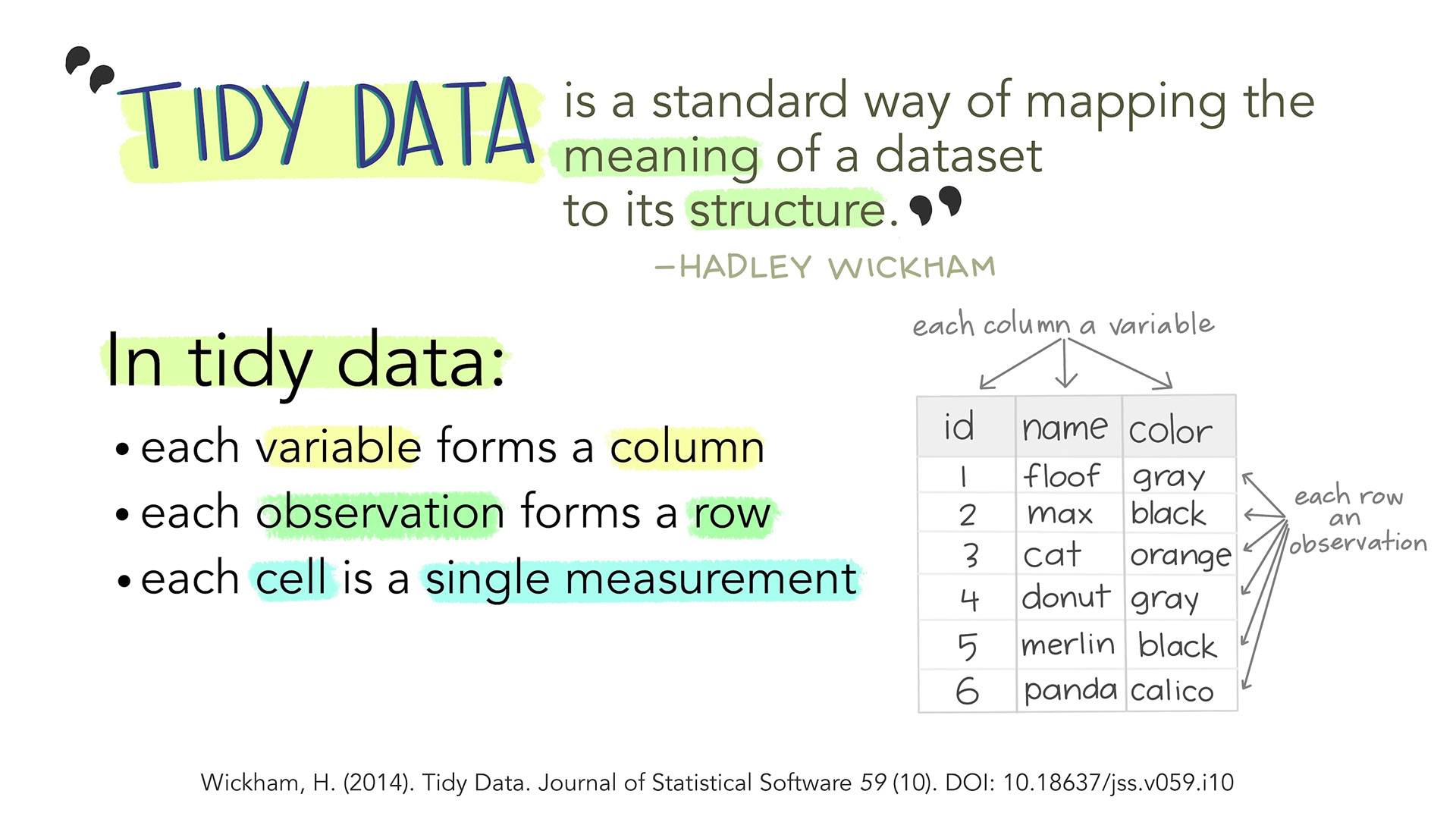
What is Tidy Data 1?

Stylized text providing an overview of Tidy Data. The top reads “Tidy data is a standard way of mapping the meaning of a dataset to its structure. - Hadley Wickham.” On the left reads “In tidy data: each variable forms a column; each observation forms a row; each cell is a single measurement.” There is an example table on the lower right with columns ‘id’, ‘name’ and ‘color’ with observations for different cats, illustrating tidy data structure.

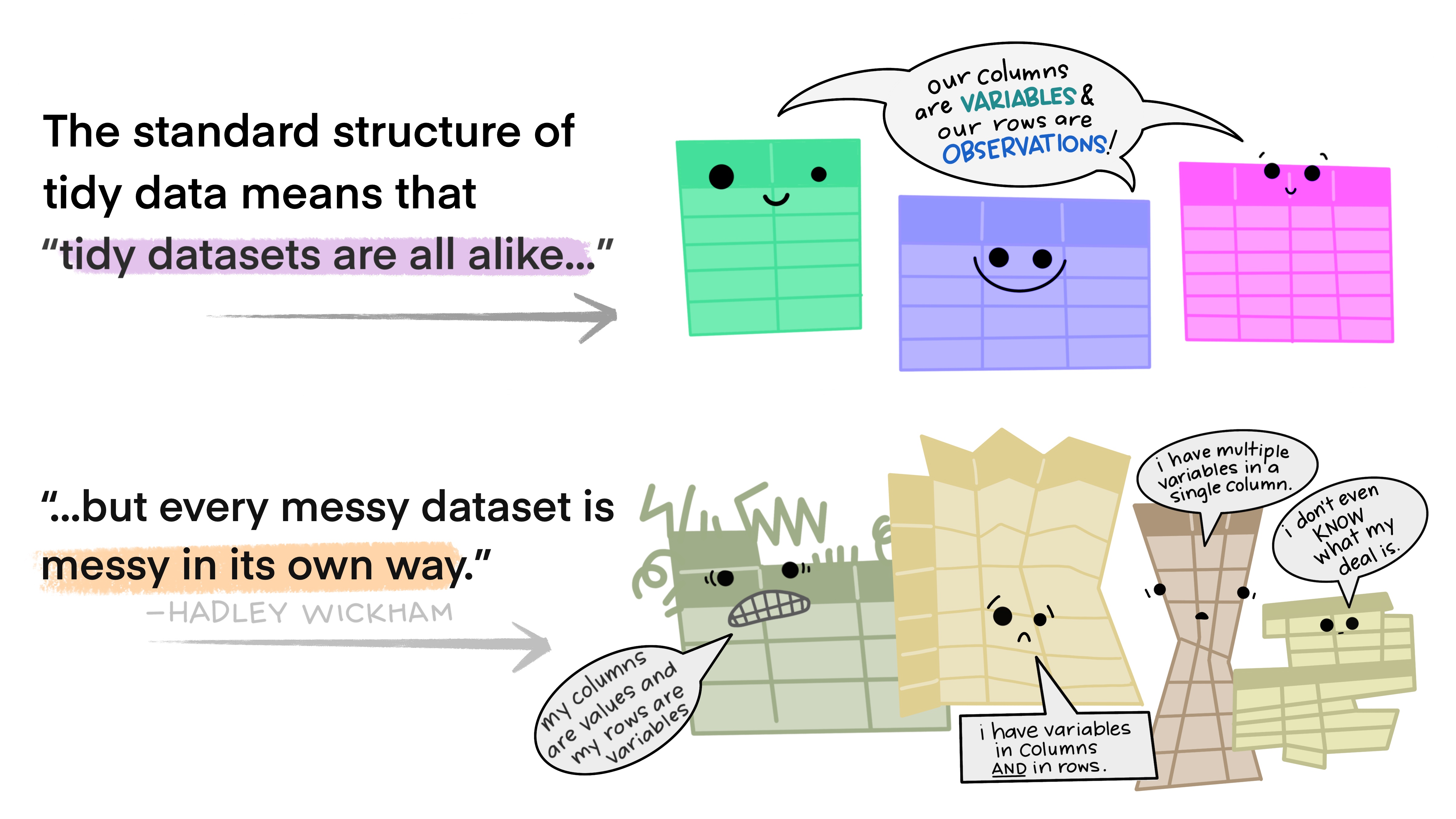
Tidy Data is predictable 1

There are two sets of anthropomorphized data tables. The top group of three tables are all rectangular and smiling, with a shared speech bubble reading “our columns are variables and our rows are observations!”. Text to the left of that group reads “The standard structure of tidy data means that “tidy datasets are all alike…” The lower group of four tables are all different shapes, look ragged and concerned, and have different speech bubbles reading (from left to right) “my column are values and my rows are variables”, “I have variables in columns AND in rows”, “I have multiple variables in a single column”, and “I don’t even KNOW what my deal is.” Next to the frazzled data tables is text “...but every messy dataset is messy in its own way. -Hadley Wickham.”

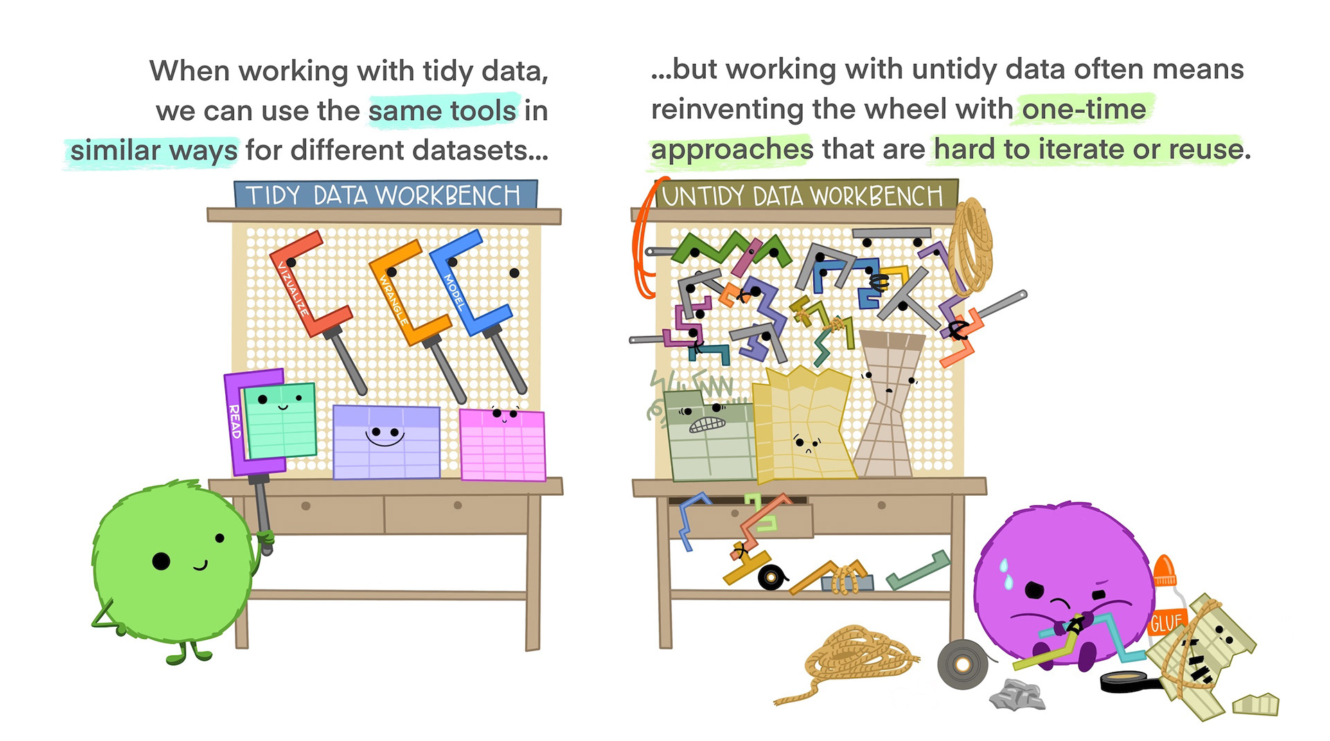
Tidy Data is more efficient 1

On the left is a happy cute fuzzy monster holding a rectangular data frame with a tool that fits the data frame shape. On the workbench behind the monster are other data frames of similar rectangular shape, and neatly arranged tools that also look like they would fit those data frames. The workbench looks uncluttered and tidy. The text above the tidy workbench reads “When working with tidy data, we can use the same tools in similar ways for different datasets…” On the right is a cute monster looking very frustrated, using duct tape and other tools to haphazardly tie data tables together, each in a different way. The monster is in front of a messy, cluttered workbench. The text above the frustrated monster reads “...but working with untidy data often means reinventing the wheel with one-time approaches that are hard to iterate or reuse.”

Why isn’t our data tidy?

month shelver stacks_books reference_books bound_journals unbound_journals
1 A 0 0 337 0
1 B 81 12 0 0
2 A 0 0 325 2
2 B 62 13 0 0
3 A 0 8 258 0
3 B 138 8 5 0
4 A 0 0 72 0
4 B 70 12 0 0

How would we plot the data?

shelving_wide %>% 
  ggplot(mapping=aes(x=???, y=???)) +
  geom_bar(stat="identity")

Wide vs long data

long data
data represented with minimum number of columns necessary, tidy data
wide data
Variables may be spread across multiple columns. Column names often represent variable values

Our Goal

month shelver material_type number_shelved
1 A stacks_books 0
1 A reference_books 0
1 A bound_journals 337
1 A unbound_journals 0
1 B stacks_books 81
1 B reference_books 12
1 B bound_journals 0
1 B unbound_journals 0
2 A stacks_books 0
2 A reference_books 0
2 A bound_journals 325
2 A unbound_journals 2
2 B stacks_books 62
2 B reference_books 13
2 B bound_journals 0
2 B unbound_journals 0
3 A stacks_books 0
3 A reference_books 8
3 A bound_journals 258
3 A unbound_journals 0
3 B stacks_books 138
3 B reference_books 8
3 B bound_journals 5
3 B unbound_journals 0
4 A stacks_books 0
4 A reference_books 0
4 A bound_journals 72
4 A unbound_journals 0
4 B stacks_books 70
4 B reference_books 12
4 B bound_journals 0
4 B unbound_journals 0

pivot_longer()

To lengthen our data, we’ll use the pivot_longer() function from the tidyr package. There are four arguments we need to provide:

  1. data - the data frame to lengthen
  2. cols - the columns we want to pivot on
  3. names_to - the name of a new column which will have our old column names as values
  4. values_to - the name of a new column which will hold the cell values of the pivoted columns