Chapter 3 Welcome to the Tidyverse
In this lesson and the next, we will be using a group of packages which are part of what is known as the tidyverse - “an opinionated collection of R packages designed for data science. All packages share an underlying design philosophy, grammar, and data structures.”6, developed by Hadley Wickham.
These packages include :
readrfor importing data into Rdplyrfor handling common data wrangling tasks for tabular datatidyrwhich enables you to swiftly convert between different data formats (long vs. wide) for plotting and analysislubridatefor working with datesggplot2for visualizing data (we’ll explore this package in the next chapter).
For the full list of tidyverse packages and documentation visit tidyverse.org You can install these packages individually, or you can install the entire tidyverse in one go.
3.1 What is Tidy Data?
Data is considered “tidy” if it follows three rules:
- Each column is a variable
- Each row is an observation
- Each cell is a single value7
Data “in the wild” often isn’t tidy, but the tidyverse packages can help you create and analyze tidy datasets.
![tidy data structure^[image from R for Data Science https://r4ds.had.co.nz/tidy-data.html#fig:tidy-structure]](images/tidy-data.png)
Figure 3.1: tidy data structure8
3.2 Getting set up
- Sign in to RStudio Cloud (Or, if you haven’t already, sign up for a free account at RStudio Cloud https://rstudio.cloud/plans/free)
- Go to the RStudio Cloud class project for this session https://rstudio.cloud/project/4266255
- Note the text that marks this as a Temporary Copy. Select the
Save a Permanent Copybutton to begin working! - Create a new script called
measles_script.R
Reminder: You can open a new R script in the following ways:
- Go to the menu bar
File > New File > R Script - In the toolbar below the menu bar, select the new blank file icon, and then R Script from the menu bar.
- In the Files pane, select the New Blank File Icon, and then R Script
- Use the keyboard shortcut
Ctrl+Shift+N(PC) orShift+Command+N(Mac)
3.3 Install
First we are going to use install.packages() to install tidyverse, if you haven’t already. Then we are going to load tidyverse with the library() function. You only need to install a package once, but you will load it each time you start a new r session. To learn more about dplyr and tidyr after the workshop, you may want to check out this handy data transformation with dplyr cheatsheet and this one about tidyr.
#install tidyverse if you haven't yet
#install.packages("tidyverse")

#load tidyverse
library(tidyverse)
## ── Attaching packages ─────────────────────────────────────── tidyverse 1.3.1 ──## ✔ ggplot2 3.3.6 ✔ purrr 0.3.4
## ✔ tibble 3.1.7 ✔ dplyr 1.0.9
## ✔ tidyr 1.2.0 ✔ stringr 1.4.0
## ✔ readr 2.1.2 ✔ forcats 0.5.1## ── Conflicts ────────────────────────────────────────── tidyverse_conflicts() ──
## ✖ dplyr::filter() masks stats::filter()
## ✖ dplyr::lag() masks stats::lag()3.4 The Data
For this lesson we will be using data which comes from Project Tycho - an open data project from the University of Pittsburgh which provides standardized datasets on numerous diseases to aid global health research.
Throughout this lesson, we will be using a dataset from Project Tycho featuring historical counts of measles cases in the U.S.. We want to clean and present this data in a way that makes it easy to see how measles cases fluctuated over time. In the next lesson, we’ll start visualizing this cleaned up data.
A useful feature of Project Tycho data is their use of a common set of variables. Read more about their data format.
3.5 Importing data
Now let’s import the data we’ll be working with. You can import data with code, or you can use RStudio’s GUI. Let’s look at both.
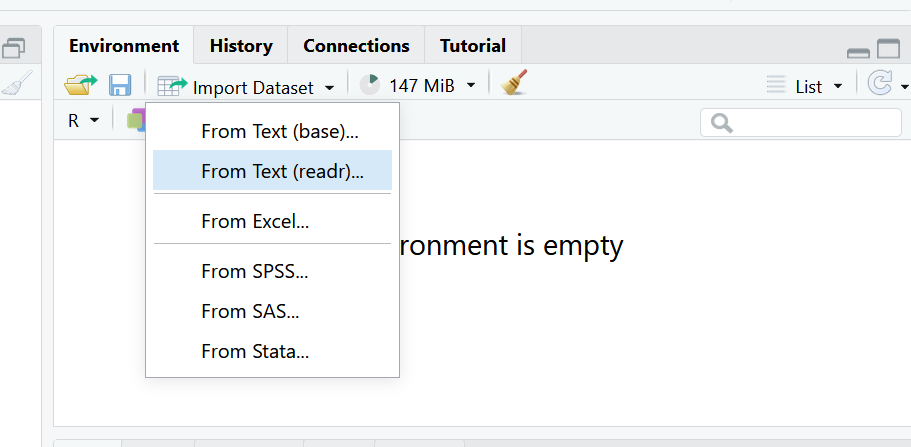
In the environment pane, select the button that says Import Dataset and choose the option From text (readr). This means we are going to be using the readr package, which is part of the tidyverse to read a file.
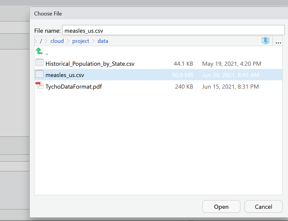
Select Browse in the dialog box that opens, and navigate to your data folder and choose the file called measles_us.csv
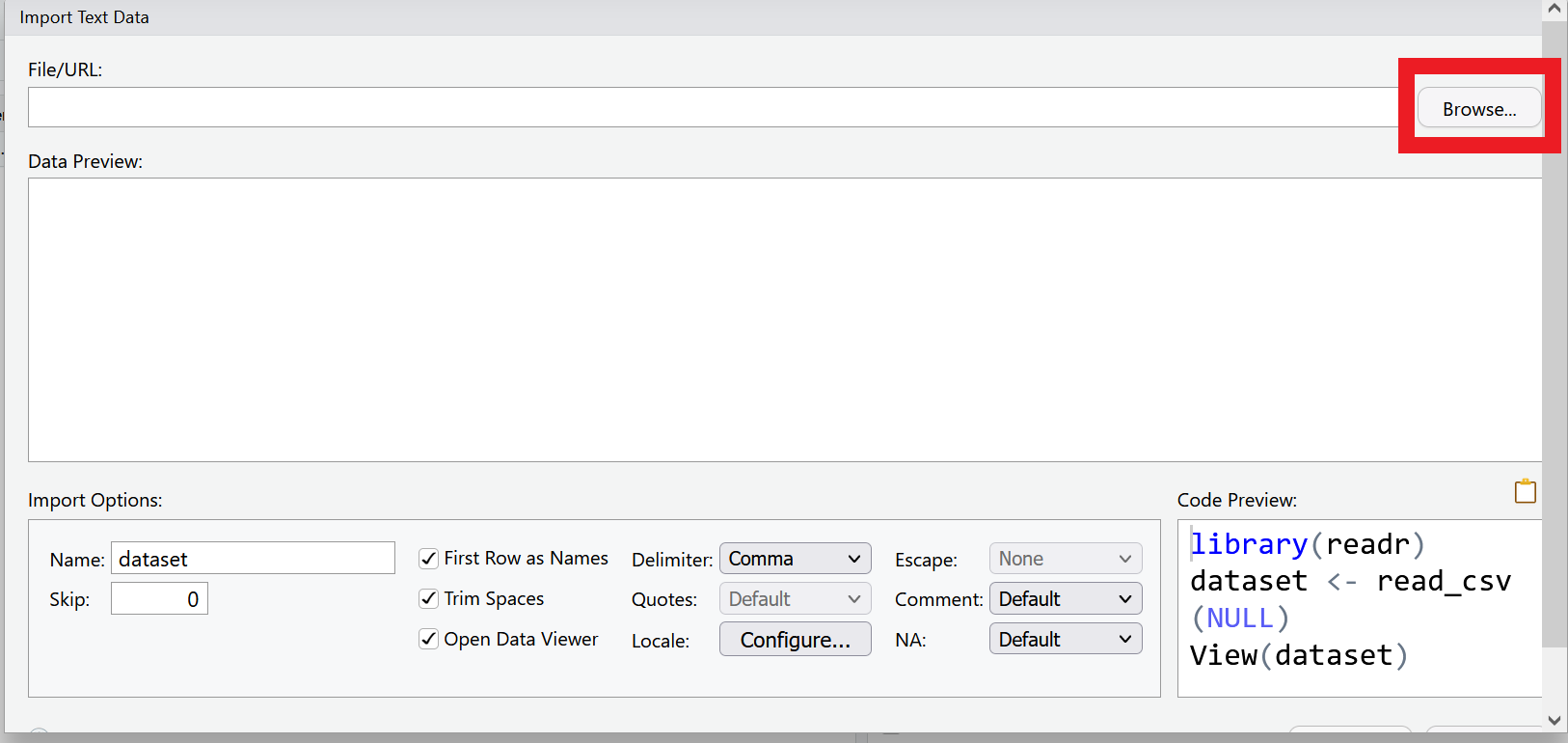
A new window will open with a spreadsheet view of the data. We can use this window to make some choices about how the data is imported.
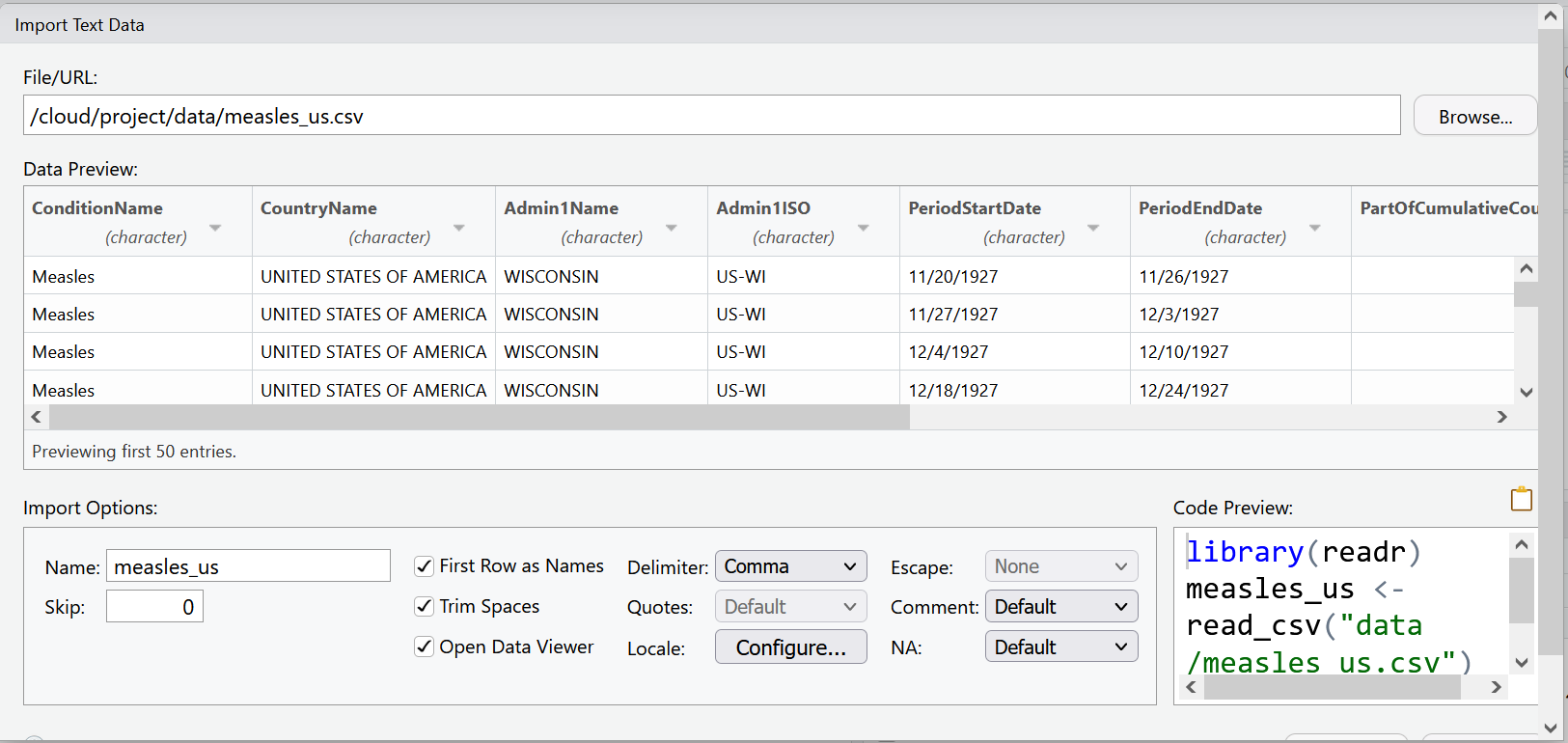
RStudio will use the file name as the default name for your dataset, but you could change it to whatever you want. In this case measles_us works pretty well.
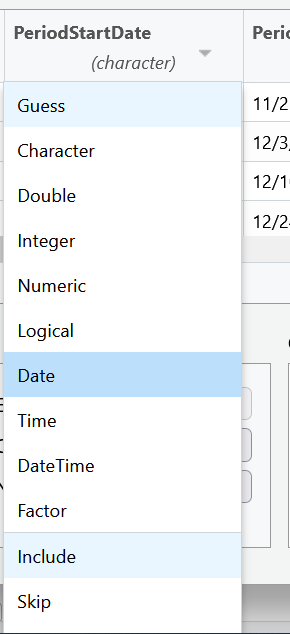
RStudio will also try to guess the data type of your columns. It will mostly get it right, but it is not unusual that you will manually need to tell it what data type certain columns are.
For example, let’s look at the columns PeriodStartDate and PeriodEndDate. These columns contain dates, but RStudio wants to read them as character data. This is very common when importing data. Let’s change the first column PeriodStartDate to the date data type, by using the drop down menu to select date data. We’ll learn another way to change data types later in this lesson and take care of PeriodEndDate then.
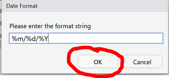
You will be asked to confirm that the input format of the date is %m/%d/%Y which is like writing mm/dd/YYYY. The program needs to know what the correct input date is so it can return the right output date YYYY-mm-dd, the international standard date format.
Now our data is ready to import. We can select the import button. As you may have noticed, the code behind this import dialog box is also being generated.
We can find the code in our History pane. Highlight the line of code and use the To Source button to add it to the script.
So what does all this code actually mean?
We are using a function from the readr package called read_csv(). This function takes as an argument the path to where the file is located. This can take the form of an absolute path, a relative path to the working directory, or a url. The col_types argument lets you specify the data type by column name.
library(readr)
measles_us <- read_csv(
  "data/measles_us.csv",
  col_types = cols(
    PeriodStartDate = col_date(format = "%m/%d/%Y")))
3.6 Exploring Data
After reading the data, you will typically want to start exploring it. There are several ways of doing this. Let’s review some ways of exploring data that we learned in the last chapter. View() opens the data as a file in your documents pane.
View(measles_us)Use summary() to look at each column
summary(measles_us)## ConditionName ConditionSNOMED PathogenName CountryName
## Length:422051 Min. :14189004 Length:422051 Length:422051
## Class :character 1st Qu.:14189004 Class :character Class :character
## Mode :character Median :14189004 Mode :character Mode :character
## Mean :14189004
## 3rd Qu.:14189004
## Max. :14189004
## CountryISO Admin1Name Admin1ISO Admin2Name
## Length:422051 Length:422051 Length:422051 Length:422051
## Class :character Class :character Class :character Class :character
## Mode :character Mode :character Mode :character Mode :character
##
##
##
## CityName PeriodStartDate PeriodEndDate
## Length:422051 Min. :1906-09-16 Length:422051
## Class :character 1st Qu.:1926-09-12 Class :character
## Mode :character Median :1940-04-07 Mode :character
## Mean :1946-02-24
## 3rd Qu.:1966-03-06
## Max. :2001-12-30
## PartOfCumulativeCountSeries DiagnosisCertainty SourceName
## Min. :0.0 Mode:logical Length:422051
## 1st Qu.:0.0 NA's:422051 Class :character
## Median :0.0 Mode :character
## Mean :0.2
## 3rd Qu.:0.0
## Max. :1.0
## CountValue
## Min. : 0.0
## 1st Qu.: 1.0
## Median : 6.0
## Mean : 136.5
## 3rd Qu.: 41.0
## Max. :53008.0You can look at the beginning of your dataset with head().
head(measles_us)## # A tibble: 6 × 15
## ConditionName Condit…¹ Patho…² Count…³ Count…⁴ Admin…⁵ Admin…⁶ Admin…⁷ CityN…⁸
## <chr> <dbl> <chr> <chr> <chr> <chr> <chr> <chr> <chr>
## 1 Measles 14189004 Measle… UNITED… US WISCON… US-WI <NA> <NA>
## 2 Measles 14189004 Measle… UNITED… US WISCON… US-WI <NA> <NA>
## 3 Measles 14189004 Measle… UNITED… US WISCON… US-WI <NA> <NA>
## 4 Measles 14189004 Measle… UNITED… US WISCON… US-WI <NA> <NA>
## 5 Measles 14189004 Measle… UNITED… US WISCON… US-WI <NA> <NA>
## 6 Measles 14189004 Measle… UNITED… US WISCON… US-WI <NA> <NA>
## # … with 6 more variables: PeriodStartDate <date>, PeriodEndDate <chr>,
## # PartOfCumulativeCountSeries <dbl>, DiagnosisCertainty <lgl>,
## # SourceName <chr>, CountValue <dbl>, and abbreviated variable names
## # ¹ConditionSNOMED, ²PathogenName, ³CountryName, ⁴CountryISO, ⁵Admin1Name,
## # ⁶Admin1ISO, ⁷Admin2Name, ⁸CityName
## # ℹ Use `colnames()` to see all variable namesor the end of your dataset with tail()
tail(measles_us)## # A tibble: 6 × 15
## ConditionName Condit…¹ Patho…² Count…³ Count…⁴ Admin…⁵ Admin…⁶ Admin…⁷ CityN…⁸
## <chr> <dbl> <chr> <chr> <chr> <chr> <chr> <chr> <chr>
## 1 Measles 14189004 Measle… UNITED… US NORTHE… US-MP <NA> <NA>
## 2 Measles 14189004 Measle… UNITED… US NORTHE… US-MP <NA> <NA>
## 3 Measles 14189004 Measle… UNITED… US NORTHE… US-MP <NA> <NA>
## 4 Measles 14189004 Measle… UNITED… US NORTHE… US-MP <NA> <NA>
## 5 Measles 14189004 Measle… UNITED… US NORTHE… US-MP <NA> <NA>
## 6 Measles 14189004 Measle… UNITED… US NORTHE… US-MP <NA> <NA>
## # … with 6 more variables: PeriodStartDate <date>, PeriodEndDate <chr>,
## # PartOfCumulativeCountSeries <dbl>, DiagnosisCertainty <lgl>,
## # SourceName <chr>, CountValue <dbl>, and abbreviated variable names
## # ¹ConditionSNOMED, ²PathogenName, ³CountryName, ⁴CountryISO, ⁵Admin1Name,
## # ⁶Admin1ISO, ⁷Admin2Name, ⁸CityName
## # ℹ Use `colnames()` to see all variable namesNotice that this prints out the first and last 6 rows of your data frame to the console in what is called a tibble. A tibble is a form of data frame that is particular to the tidyverse. The differences rest mainly it how it reads and displays data, but for the purposes of this class we will use the terms somewhat interchangeably. The tibble printed from head() and tail() will only print as many columns as can fit on the width of your monitor.
The glimpse() function which is part of the tidyverse package tibble, lets you see the column names and data types clearly.
#summary of columns and first few entries
glimpse(measles_us)
## Rows: 422,051
## Columns: 15
## $ ConditionName <chr> "Measles", "Measles", "Measles", "Measles"…
## $ ConditionSNOMED <dbl> 14189004, 14189004, 14189004, 14189004, 14…
## $ PathogenName <chr> "Measles virus", "Measles virus", "Measles…
## $ CountryName <chr> "UNITED STATES OF AMERICA", "UNITED STATES…
## $ CountryISO <chr> "US", "US", "US", "US", "US", "US", "US", …
## $ Admin1Name <chr> "WISCONSIN", "WISCONSIN", "WISCONSIN", "WI…
## $ Admin1ISO <chr> "US-WI", "US-WI", "US-WI", "US-WI", "US-WI…
## $ Admin2Name <chr> NA, NA, NA, NA, NA, NA, NA, NA, NA, NA, NA…
## $ CityName <chr> NA, NA, NA, NA, NA, NA, NA, NA, NA, NA, NA…
## $ PeriodStartDate <date> 1927-11-20, 1927-11-27, 1927-12-04, 1927-…
## $ PeriodEndDate <chr> "11/26/1927", "12/3/1927", "12/10/1927", "…
## $ PartOfCumulativeCountSeries <dbl> 0, 0, 0, 0, 0, 0, 0, 0, 0, 0, 0, 0, 0, 0, …
## $ DiagnosisCertainty <lgl> NA, NA, NA, NA, NA, NA, NA, NA, NA, NA, NA…
## $ SourceName <chr> "US Nationally Notifiable Disease Surveill…
## $ CountValue <dbl> 85, 120, 84, 106, 39, 45, 28, 140, 48, 85,…Some of our variables only have one value. For example ConditionName is always going to be “Measles” and CountryName is always going to be “UNITED STATES OF AMERICA”, because this dataset is a dataset of measles case counts in the US. But you don’t have to take my word for it! Let’s use some tools to explore distinct values. First the dplyr function distinct() will print all the distinct values in a given column.
distinct(measles_us, ConditionName)## # A tibble: 1 × 1
## ConditionName
## <chr>
## 1 MeaslesAs expected, we have only one distinct value in this column.
To contrast, let’s run distinct() on Admin1Name.
distinct(measles_us, Admin1Name)## # A tibble: 56 × 1
## Admin1Name
## <chr>
## 1 WISCONSIN
## 2 OHIO
## 3 MICHIGAN
## 4 NEVADA
## 5 NEW JERSEY
## 6 WASHINGTON
## 7 DELAWARE
## 8 KENTUCKY
## 9 WYOMING
## 10 INDIANA
## # … with 46 more rows
## # ℹ Use `print(n = ...)` to see more rowsNow we get a clearer idea that this column contains names of US states and territories.
We might want, not just the distinct values, but also counts of how often each distinct value occurs. For that we can use count()
count(measles_us, Admin1Name)## # A tibble: 56 × 2
## Admin1Name n
## <chr> <int>
## 1 ALABAMA 7458
## 2 ALASKA 1869
## 3 AMERICAN SAMOA 118
## 4 ARIZONA 4685
## 5 ARKANSAS 5643
## 6 CALIFORNIA 14354
## 7 COLORADO 8042
## 8 CONNECTICUT 10816
## 9 DELAWARE 4507
## 10 DISTRICT OF COLUMBIA 5027
## # … with 46 more rows
## # ℹ Use `print(n = ...)` to see more rowsThis might be helpful information to have on its own. Let’s save this to an object that we can refer to later.
Admin1_counts <- count(measles_us, Admin1Name)We might also notice that some of our columns have a number of NA values. Let’s take a closer look at one of these. We can use the function is.na() to test for the presence of NAs in our data. is.na() will return a vector of values TRUE or FALSE. TRUE if the value is NA, FALSE if it is not.
is.na(measles_us$Admin2Name)We can use that together with sum() to find out how many NAs are in the column.
sum(is.na(measles_us$Admin2Name))## [1] 198104To find out how many NAs there are per column of our dataset, we can use the function colSums().
colSums(is.na(measles_us))## ConditionName ConditionSNOMED
## 0 0
## PathogenName CountryName
## 0 0
## CountryISO Admin1Name
## 0 0
## Admin1ISO Admin2Name
## 0 198104
## CityName PeriodStartDate
## 198104 0
## PeriodEndDate PartOfCumulativeCountSeries
## 0 0
## DiagnosisCertainty SourceName
## 422051 0
## CountValue
## 0We see that Admin2Name and CityName variables have many missing values, and the DiagnosisCertainty column is entirely missing (i.e. the number of missing values is the same as the number of observations in the dataset). This is something to consider as we figure out what variables we want to focus our analysis on.
3.6.1 Challenge
- Test out
distinct()with a few other columns inmeasles_us. unique()andtable()are two base R functions that work similarly todistinct()andcount(). Try runningunique(measles_us$Admin1Name)andtable(measles_us$Admin1Name). How do the results differ fromdistinct()andcount()? Which do you prefer?- Try to run
unique()andtable()on a few more variables in measles_us() - Look up the
colSums()in RStudio Help pane. What are some related functions and what do they do? Test them out!
3.7 Wrangling data with dplyr
Now that we have a better sense of what’s in our data, we can start to getting it into shape for analysis. Of all the tidyverse packages, dplyr might be the one you wind up using the most. dplyr is characterized by its easy to understand “verb” functions, such as count(), which we’ve already used. Some others are:
select()- selects columns by namefilter()- filters rows by some conditionmutate()- creates new columns based on existing values of existing columnsgroup_by()- groups datasummarize()- summarizes rows to a single valuearrange()- changes the order of rows
If you’re familiar at all with SQL, you may that some of these dplyr functions have similar names or purposes as SQL commands.
3.8 Subsetting Data
To work efficiently, we want to work with the smallest version of our dataset possible that still contains all the information we need. That means getting rid of extraneous columns and rows. In the last chapter, we learned that we can use brackets to subset vectors and data frames.
For example:
# use bracket notation to select the value in the 5th row, 7th column
measles_us[5,7]
## # A tibble: 1 × 1
## Admin1ISO
## <chr>
## 1 US-WI
#use bracket notation to select the 3rd row
measles_us[3,]
## # A tibble: 1 × 15
## ConditionName Condit…¹ Patho…² Count…³ Count…⁴ Admin…⁵ Admin…⁶ Admin…⁷ CityN…⁸
## <chr> <dbl> <chr> <chr> <chr> <chr> <chr> <chr> <chr>
## 1 Measles 14189004 Measle… UNITED… US WISCON… US-WI <NA> <NA>
## # … with 6 more variables: PeriodStartDate <date>, PeriodEndDate <chr>,
## # PartOfCumulativeCountSeries <dbl>, DiagnosisCertainty <lgl>,
## # SourceName <chr>, CountValue <dbl>, and abbreviated variable names
## # ¹ConditionSNOMED, ²PathogenName, ³CountryName, ⁴CountryISO, ⁵Admin1Name,
## # ⁶Admin1ISO, ⁷Admin2Name, ⁸CityName
## # ℹ Use `colnames()` to see all variable names
#use bracket notation to select the 10th column
measles_us[10]
## # A tibble: 422,051 × 1
## PeriodStartDate
## <date>
## 1 1927-11-20
## 2 1927-11-27
## 3 1927-12-04
## 4 1927-12-18
## 5 1927-12-25
## 6 1928-01-01
## 7 1928-01-08
## 8 1928-01-15
## 9 1928-01-22
## 10 1928-01-29
## # … with 422,041 more rows
## # ℹ Use `print(n = ...)` to see more rows
#use bracket notation to select a range of rows and columns
measles_us[6:10, 3:9]
## # A tibble: 5 × 7
## PathogenName CountryName Count…¹ Admin…² Admin…³ Admin…⁴ CityN…⁵
## <chr> <chr> <chr> <chr> <chr> <chr> <chr>
## 1 Measles virus UNITED STATES OF AMERICA US WISCON… US-WI <NA> <NA>
## 2 Measles virus UNITED STATES OF AMERICA US WISCON… US-WI <NA> <NA>
## 3 Measles virus UNITED STATES OF AMERICA US WISCON… US-WI <NA> <NA>
## 4 Measles virus UNITED STATES OF AMERICA US WISCON… US-WI <NA> <NA>
## 5 Measles virus UNITED STATES OF AMERICA US WISCON… US-WI <NA> <NA>
## # … with abbreviated variable names ¹CountryISO, ²Admin1Name, ³Admin1ISO,
## # ⁴Admin2Name, ⁵CityName3.8.1 Subsetting Columns with Select()
dplyr makes this subsetting task a bit easier, because we can use select() to choose columns by name rather than index.
The first argument to this function is the name of the data object, which in this case is measles_us, and the subsequent arguments are the names of the columns we want to keep, separated by commas.
Let’s try selecting the Admin1Name column and the CountValue column.
select(measles_us, Admin1Name, CountValue)## # A tibble: 422,051 × 2
## Admin1Name CountValue
## <chr> <dbl>
## 1 WISCONSIN 85
## 2 WISCONSIN 120
## 3 WISCONSIN 84
## 4 WISCONSIN 106
## 5 WISCONSIN 39
## 6 WISCONSIN 45
## 7 WISCONSIN 28
## 8 WISCONSIN 140
## 9 WISCONSIN 48
## 10 WISCONSIN 85
## # … with 422,041 more rows
## # ℹ Use `print(n = ...)` to see more rowsAs you can imagine, if you had a number of columns to select, it could get tiresome to write them all out. One way around this is to use a colon : to name a range of adjacent columns, just as we used the colon with brackets.
select(measles_us, ConditionName:Admin1ISO)## # A tibble: 422,051 × 7
## ConditionName ConditionSNOMED PathogenName Country…¹ Count…² Admin…³ Admin…⁴
## <chr> <dbl> <chr> <chr> <chr> <chr> <chr>
## 1 Measles 14189004 Measles virus UNITED S… US WISCON… US-WI
## 2 Measles 14189004 Measles virus UNITED S… US WISCON… US-WI
## 3 Measles 14189004 Measles virus UNITED S… US WISCON… US-WI
## 4 Measles 14189004 Measles virus UNITED S… US WISCON… US-WI
## 5 Measles 14189004 Measles virus UNITED S… US WISCON… US-WI
## 6 Measles 14189004 Measles virus UNITED S… US WISCON… US-WI
## 7 Measles 14189004 Measles virus UNITED S… US WISCON… US-WI
## 8 Measles 14189004 Measles virus UNITED S… US WISCON… US-WI
## 9 Measles 14189004 Measles virus UNITED S… US WISCON… US-WI
## 10 Measles 14189004 Measles virus UNITED S… US WISCON… US-WI
## # … with 422,041 more rows, and abbreviated variable names ¹CountryName,
## # ²CountryISO, ³Admin1Name, ⁴Admin1ISO
## # ℹ Use `print(n = ...)` to see more rowsAnother helpful tool that the tidyverse provides is the pipe operator which looks like %>%. The pipe is made available via the magrittr package, installed automatically with dplyr. If you use RStudio, you can type the pipe with Ctrl + Shift + M if you have a PC or Cmd + Shift + M if you have a Mac.
With the pipe you start with your data object and pipe it to the function, rather than naming the data as your first argument. So, the pipe becomes especially valuable when you have a number of steps that you want to connect. Another benefit of using the pipe in RStudio is that the interface will supply column names to you in the auto complete. This helps so you do not need to remember sometimes lengthy column names, and you are less likely to get an error from a typo.
measles_us %>%
  select(Admin1Name, PartOfCumulativeCountSeries)
## # A tibble: 422,051 × 2
## Admin1Name PartOfCumulativeCountSeries
## <chr> <dbl>
## 1 WISCONSIN 0
## 2 WISCONSIN 0
## 3 WISCONSIN 0
## 4 WISCONSIN 0
## 5 WISCONSIN 0
## 6 WISCONSIN 0
## 7 WISCONSIN 0
## 8 WISCONSIN 0
## 9 WISCONSIN 0
## 10 WISCONSIN 0
## # … with 422,041 more rows
## # ℹ Use `print(n = ...)` to see more rowsNow, let’s think through which columns we want for our analysis and save this to a new object called measles_us_mod. It’s always a good idea to create new objects when you make major changes to your data.
For this exercise, we want to look at trends in number of measles cases over time. To do that, we’ll need to keep our CountValue variable, as and the date variables (PeriodStartDate and PeriodEndDate), as well as thePartOfCumulativeCountSeries variable, which will help us understand how to use the dates (more on this later). The first five columns each have only one value. So it might be redundant to keep those, although if we were combining them with other Project Tycho datasets they could be useful. It might be interesting to get a state-level view of the data, so let’s keep Admin1Name. But we saw that there are a number of missing values in our Admin2Name and CityName variables, so they might not be very useful for our analysis.
measles_us_mod <-
  measles_us %>%
    select(
     Admin1Name,
     PeriodStartDate,
     PeriodEndDate,
     PartOfCumulativeCountSeries,
     CountValue
)

# inspect our new data frame
glimpse(measles_us_mod)
## Rows: 422,051
## Columns: 5
## $ Admin1Name <chr> "WISCONSIN", "WISCONSIN", "WISCONSIN", "WI…
## $ PeriodStartDate <date> 1927-11-20, 1927-11-27, 1927-12-04, 1927-…
## $ PeriodEndDate <chr> "11/26/1927", "12/3/1927", "12/10/1927", "…
## $ PartOfCumulativeCountSeries <dbl> 0, 0, 0, 0, 0, 0, 0, 0, 0, 0, 0, 0, 0, 0, …
## $ CountValue <dbl> 85, 120, 84, 106, 39, 45, 28, 140, 48, 85,…Now when you look in your environment pane, you should see your new object which as the same number of rows but 6 instead of 11 columns (or variables)
3.8.2 Renaming columns
Sometimes when you receive data, you may find that the column names are not very descriptive or useful, and it may be necessary to rename them. You can assign new names to columns when you select them select(newColumnName = OldColumnName) or you can use the rename() function. Like naming objects, you should use a simple, descriptive, relatively short name without spaces for your column names.
measles_us_mod <-
  measles_us_mod %>%
    rename(State = Admin1Name)
3.8.3 Subsetting rows with filter()
select() lets us choose columns. To choose rows based on a specific criteria, we can use the filter() function. The arguments after the data frame are the condition(s) we want for our final dataframe to adhere to. Specify conditions using logical operator:
| operator | meaning |
|---|---|
| == | exactly equal |
| != | not equal to |
| < | less than |
| <= | less than or equal to |
| > | greater than |
| >= | greater than or equal to |
| x|y | x or y |
| x&y | x and y |
| !x | not x |
We’ll come back to our problem of different time spans in a moment. First, let’s try filtering our data by just one condition. We want to see just the rows that contain counts from Maryland.
measles_us_mod %>% filter(State == "MARYLAND")## # A tibble: 7,246 × 5
## State PeriodStartDate PeriodEndDate PartOfCumulativeCountSeries CountValue
## <chr> <date> <chr> <dbl> <dbl>
## 1 MARYLAND 1927-11-27 12/3/1927 0 64
## 2 MARYLAND 1927-12-04 12/10/1927 0 88
## 3 MARYLAND 1927-12-18 12/24/1927 0 105
## 4 MARYLAND 1927-12-25 12/31/1927 0 109
## 5 MARYLAND 1928-01-01 1/7/1928 0 175
## 6 MARYLAND 1928-01-08 1/14/1928 0 249
## 7 MARYLAND 1928-01-15 1/21/1928 0 345
## 8 MARYLAND 1928-01-22 1/28/1928 0 365
## 9 MARYLAND 1928-01-29 2/4/1928 0 504
## 10 MARYLAND 1928-02-05 2/11/1928 0 563
## # … with 7,236 more rows
## # ℹ Use `print(n = ...)` to see more rowsWhen matching strings you must be exact. R is case-sensitive. So State == "Maryland" or State == "maryland" would return 0 rows.
You can add additional conditions to filter by, separated by commas or other logical operators like &, >, and >.
Below we want just the rows for Maryland, and only include periods where the count was more than 500 reported cases. Note that while you need quotation marks around character data, you do not need them around numeric data.
measles_us_mod %>%
  filter(State == "MARYLAND" & CountValue > 500)
## # A tibble: 328 × 5
## State PeriodStartDate PeriodEndDate PartOfCumulativeCountSeries CountValue
## <chr> <date> <chr> <dbl> <dbl>
## 1 MARYLAND 1928-01-29 2/4/1928 0 504
## 2 MARYLAND 1928-02-05 2/11/1928 0 563
## 3 MARYLAND 1928-02-12 2/18/1928 0 696
## 4 MARYLAND 1928-02-19 2/25/1928 0 750
## 5 MARYLAND 1928-02-26 3/3/1928 0 1012
## 6 MARYLAND 1928-03-04 3/10/1928 0 951
## 7 MARYLAND 1928-03-11 3/17/1928 0 1189
## 8 MARYLAND 1928-03-18 3/24/1928 0 1163
## 9 MARYLAND 1928-03-25 3/31/1928 0 1020
## 10 MARYLAND 1928-04-01 4/7/1928 0 753
## # … with 318 more rows
## # ℹ Use `print(n = ...)` to see more rowsWe can filter based on a vector of values with the%in% operator. Remember that our dataset contains data for US states and territories. To do this we will make use of a nifty built-in R vector called state.name. We’ll keep only the rows where the State column has a value that matches one of the values in that vector. Because the state names in our data are in all upper case letters, we will use the base R function toupper() (to upper case).
measles_states_only <-
  measles_us_mod %>%
  filter(State %in% toupper(state.name))
Let’s save this output to a new object measles_states_only. Notice how we now have fewer rows than we had in our measles_us_mod object.
We could alternatively have used negation with the names of the values we specifically wanted to exclude.
measles_states_only <- measles_us_mod %>%
  filter(!State %in% c("PUERTO RICO", "GUAM", "AMERICAN SAMOA", "NORTHERN MARIANA ISLANDS", "VIRGIN ISLANDS, U.S.", "DISTRICT OF COLUMBIA"))
Great! Our dataset is really shaping up. Let’s also take a closer look at our date columns. If you look at the first several rows, it looks like each row of our dataset represents about a discrete week of measles case counts. But (as you can read in the Tycho data documentation) there are actually two date series in this dataset - non-cumulative and cumulative. Which series a row belongs to is noted by the PartofCumulativeCountSeries, which as the value 0 if a row is non-cumulative, and 1 if the row is part of a cumulative count.
To keep things consistent. Let’s filter our dataset so we only have the non-overlapping discrete weeks.
measles_non_cumulative <-
  measles_states_only %>%
  filter(PartOfCumulativeCountSeries==0)
Once again, we have fewer rows than we started with.
3.9 Working with Dates
Working with dates in your dataset can be tricky. The tidyverse provides the lubridate package to make this task easier. Because of it’s specialized focus, it’s not loaded with the rest of the tidyverse packages. So let’s load it now:
library(lubridate)##
## Attaching package: 'lubridate'## The following objects are masked from 'package:base':
##
## date, intersect, setdiff, unionAs we saw when we loaded our measles dataset, R often will try to read in date variables as character data. But, if we want to be able to do calculations with our dates, or graph some time information, we need the dates to be recognized as date objects.
lubridate has a number of functions for parsing and creating dates. Let’s say we have a character string that looks like a date in a typical US date format: month, day, year. We can parse this with the function called mdy()
my_date <- "03/14/2022"
real_date <- mdy(my_date)

real_date
## [1] "2022-03-14"Note it changes the date to a standard format Year-Month-Day. Let’s look at the classes of our two dates.
class(my_date)
## [1] "character"
class(real_date)
## [1] "Date"
Let’s try parsing a couple more dates in different formats with related functions dmy() and ymd():
dmy("14-03-2022")
## [1] "2022-03-14"
ymd("20220314")
## [1] "2022-03-14"
Note that you can use different types of separators between the date components or no separators at all.
Now let’s use this new function to change PeriodEndDate to a date object. Currently, the dates are in Month, Day, Year format. Notice that since we are changing one column of data, we must save the results of our function directly to that column. We can use the class() function to check that it worked.
measles_non_cumulative$PeriodEndDate <- mdy(measles_non_cumulative$PeriodEndDate)

class(measles_non_cumulative$PeriodEndDate)
## [1] "Date"lubridate also has functions that will let you pull out different components of dates. For example:
year(real_date)
## [1] 2022
month(real_date)
## [1] 3
day(real_date)
## [1] 14
wday(real_date)
## [1] 2
wday(real_date, label = TRUE)
## [1] Mon
## Levels: Sun < Mon < Tue < Wed < Thu < Fri < Sat
We’ll come back to that idea shortly.
3.9.1 Date intervals, durations, and periods
We can also use lubridate to work with time durations, intervals, and periods, and to do arithmetic with dates.
The measles data has a start date and an end date variable. This dataset has a mix of discrete 6 day periods and cumulative periods. Let’s look at that a little more closely. First we create an interval object based on those two dates with the interval() function.
measles_weeks <- measles_us_mod

measles_weeks$PeriodEndDate <- mdy(measles_weeks$PeriodEndDate)

measles_intervals <-
  interval(start=measles_weeks$PeriodStartDate, end=measles_weeks$PeriodEndDate)

head(measles_intervals)
## [1] 1927-11-20 UTC--1927-11-26 UTC 1927-11-27 UTC--1927-12-03 UTC
## [3] 1927-12-04 UTC--1927-12-10 UTC 1927-12-18 UTC--1927-12-24 UTC
## [5] 1927-12-25 UTC--1927-12-31 UTC 1928-01-01 UTC--1928-01-07 UTCTo figure out how many days are in our interval we can use a duration function. Duration functions return the number of seconds in a provided value.
duration(10)
## [1] "10s"
dminutes(10)
## [1] "600s (~10 minutes)"
dhours(10)
## [1] "36000s (~10 hours)"
ddays(10)
## [1] "864000s (~1.43 weeks)"
measles_days <-
measles_intervals / ddays(1)
head(measles_days)## [1] 6 6 6 6 6 6The table function will tell us how many times each interval appears
as_tibble(table(measles_days))## # A tibble: 59 × 2
## measles_days n
## <chr> <int>
## 1 6 338063
## 2 13 558
## 3 20 693
## 4 27 782
## 5 34 857
## 6 41 929
## 7 48 913
## 8 55 997
## 9 62 1083
## 10 69 1136
## # … with 49 more rows
## # ℹ Use `print(n = ...)` to see more rows3.10 Creating new columns with mutate()
Frequently you’ll want to create new columns based on the values in existing columns, for example to do unit conversions, or to find the ratio of values in two columns. For this you can use the mutate() function. The transmute() function is similar, but replaces old columns with the new one.
We can use mutate() plus what we learned about lubridate functions to create a Year variable based on our current date variables. This will be useful later on for grouping purposes. mutate() takes as an argument the name of the new column you want to create and an expression used to create it.
measles_w_year <-
  measles_non_cumulative %>%
  mutate(Year=year(PeriodStartDate))

glimpse(measles_w_year)
## Rows: 332,138
## Columns: 6
## $ State <chr> "WISCONSIN", "WISCONSIN", "WISCONSIN", "WI…
## $ PeriodStartDate <date> 1927-11-20, 1927-11-27, 1927-12-04, 1927-…
## $ PeriodEndDate <date> 1927-11-26, 1927-12-03, 1927-12-10, 1927-…
## $ PartOfCumulativeCountSeries <dbl> 0, 0, 0, 0, 0, 0, 0, 0, 0, 0, 0, 0, 0, 0, …
## $ CountValue <dbl> 85, 120, 84, 106, 39, 45, 28, 140, 48, 85,…
## $ Year <dbl> 1927, 1927, 1927, 1927, 1927, 1928, 1928, …3.11 Grouping and Summarizing data
Many data analysis tasks can be approached using the split-apply-combine paradigm: split the data into groups, apply some analysis to each group, and then combine the results. dplyr makes this very easy through the use of the group_by() function.
group_by() is often used together with summarize(), which collapses each group into a single-row summary of that group. group_by() takes as arguments the column names that contain the categorical variables for which you want to calculate the summary statistics.
How can we calculate the total number of measles cases for each year?
First we need to group our data by year using our new Year column.
yearly_count_state <-
  measles_w_year %>%
  group_by(Year)

head(yearly_count_state)
## # A tibble: 6 × 6
## # Groups: Year [2]
## State PeriodStartDate PeriodEndDate PartOfCumulativeCountS…¹ Count…² Year
## <chr> <date> <date> <dbl> <dbl> <dbl>
## 1 WISCONSIN 1927-11-20 1927-11-26 0 85 1927
## 2 WISCONSIN 1927-11-27 1927-12-03 0 120 1927
## 3 WISCONSIN 1927-12-04 1927-12-10 0 84 1927
## 4 WISCONSIN 1927-12-18 1927-12-24 0 106 1927
## 5 WISCONSIN 1927-12-25 1927-12-31 0 39 1927
## 6 WISCONSIN 1928-01-01 1928-01-07 0 45 1928
## # … with abbreviated variable names ¹PartOfCumulativeCountSeries, ²CountValueWhen you inspect your new data frame, everything should look the same. Grouping prepares your data for summarize, but it does not do anything visually to the data.
Now let’s trying summarizing that data. summarize() condenses the value of the group values to a single value per group. Like mutate(), we provide the function with the name of the new column that will hold the summary information. In this case, we will use the sum() function on the CountValue column and put this in a new column called TotalCount. Summarize will drop the columns that aren’t being used.
#Get totals for each state each year.
yearly_count <-
  measles_w_year %>%
  group_by(Year) %>%
  summarise(TotalCount = sum(CountValue))

head(yearly_count)
## # A tibble: 6 × 2
## Year TotalCount
## <dbl> <dbl>
## 1 1906 2345
## 2 1907 40199
## 3 1908 54471
## 4 1909 49802
## 5 1910 86984
## 6 1911 59171A more useful view might be to look for yearly totals of case counts by state. We can group by two variables, Year, and then State.
#Get totals for each state each year.
yearly_count_state <-
  measles_w_year %>%
  group_by(Year, State) %>%
  summarise(TotalCount = sum(CountValue))
## `summarise()` has grouped output by 'Year'. You can override using the
## `.groups` argument.head(yearly_count_state)## # A tibble: 6 × 3
## # Groups: Year [1]
## Year State TotalCount
## <dbl> <chr> <dbl>
## 1 1906 CALIFORNIA 224
## 2 1906 CONNECTICUT 23
## 3 1906 FLORIDA 4
## 4 1906 ILLINOIS 187
## 5 1906 INDIANA 20
## 6 1906 KENTUCKY 2Notice how the use of pipes really comes in handy here. It saved us from having to create and keep track of a number of intermediate objects.
3.12 Sorting datasets with arrange()
Which state in which year had the highest case count? To easily find out, we can use the function arrange(). One of the arguments must be the column you want to sort on.
yearly_count_state %>% arrange(TotalCount)## # A tibble: 4,055 × 3
## # Groups: Year [96]
## Year State TotalCount
## <dbl> <chr> <dbl>
## 1 1925 NEVADA 0
## 2 1937 MISSISSIPPI 0
## 3 1938 MISSISSIPPI 0
## 4 1939 MISSISSIPPI 0
## 5 1940 MISSISSIPPI 0
## 6 1940 NEVADA 0
## 7 1941 MISSISSIPPI 0
## 8 1944 MISSISSIPPI 0
## 9 1945 MISSISSIPPI 0
## 10 1906 TEXAS 1
## # … with 4,045 more rows
## # ℹ Use `print(n = ...)` to see more rowsBy default, arrange sorts in ascending order. To sort by descending order we use together with the desc() function.
yearly_count_state %>% arrange(desc(TotalCount))## # A tibble: 4,055 × 3
## # Groups: Year [96]
## Year State TotalCount
## <dbl> <chr> <dbl>
## 1 1938 PENNSYLVANIA 146467
## 2 1941 PENNSYLVANIA 137180
## 3 1938 ILLINOIS 127935
## 4 1942 CALIFORNIA 116180
## 5 1941 OHIO 114788
## 6 1935 MICHIGAN 111413
## 7 1941 NEW YORK 109663
## 8 1938 MICHIGAN 109041
## 9 1934 PENNSYLVANIA 107031
## 10 1938 WISCONSIN 104450
## # … with 4,045 more rows
## # ℹ Use `print(n = ...)` to see more rows3.13 Joining Datasets
Of course, looking at total counts in each state is not the most helpful metric without taking population into account. To rectify this, let’s try joining some historical population data with our measles data.
First we need to import the population data9. In addition to importing a file on your computer, you can also import data using a url to download data from the internet directly to your R session.
#load csv of populations by state over time, changing some of the datatypes from default
hist_pop_by_state <-
  read_csv(
    "https://osf.io/download/62cdb7d8779f1710fb070f06/")
## Rows: 107 Columns: 52
## ── Column specification ────────────────────────────────────────────────────────
## Delimiter: ","
## dbl (52): DATE, ALASKA, ALABAMA, ARKANSAS, ARIZONA, CALIFORNIA, COLORADO, CO...
##
## ℹ Use `spec()` to retrieve the full column specification for this data.
## ℹ Specify the column types or set `show_col_types = FALSE` to quiet this message.head(hist_pop_by_state)## # A tibble: 6 × 52
## DATE ALASKA ALABAMA ARKANSAS ARIZONA CALIFO…¹ COLOR…² CONNE…³ DISTR…⁴ DELAW…⁵
## <dbl> <dbl> <dbl> <dbl> <dbl> <dbl> <dbl> <dbl> <dbl> <dbl>
## 1 1900 NA 1830 1314 124 1490 543 910 278 185
## 2 1901 NA 1907 1341 131 1550 581 931 285 187
## 3 1902 NA 1935 1360 138 1623 621 952 290 188
## 4 1903 NA 1957 1384 144 1702 652 972 295 190
## 5 1904 NA 1978 1419 151 1792 659 987 302 192
## 6 1905 NA 2012 1447 158 1893 680 1010 308 194
## # … with 42 more variables: FLORIDA <dbl>, GEORGIA <dbl>, HAWAII <dbl>,
## # IOWA <dbl>, IDAHO <dbl>, ILLINOIS <dbl>, INDIANA <dbl>, KANSAS <dbl>,
## # KENTUCKY <dbl>, LOUISIANA <dbl>, MASSACHUSETTS <dbl>, MARYLAND <dbl>,
## # MAINE <dbl>, MICHIGAN <dbl>, MINNESOTA <dbl>, MISSOURI <dbl>,
## # MISSISSIPPI <dbl>, MONTANA <dbl>, `NORTH CAROLINA` <dbl>,
## # `NORTH DAKOTA` <dbl>, NEBRASKA <dbl>, `NEW HAMPSHIRE` <dbl>,
## # `NEW JERSEY` <dbl>, `NEW MEXICO` <dbl>, NEVADA <dbl>, `NEW YORK` <dbl>, …
## # ℹ Use `colnames()` to see all variable namesView(hist_pop_by_state)3.13.1 Long vs Wide formats
Remember that for data to be considered “tidy”, it should be in what is called “long” format. Each column is a variable, each row is an observation, and each cell is a value. Our state population data is in “wide” format, because State Name is being treated as a variable, when it is really a value. Wide data is often preferable for human-readability, but is less ideal for machine-readability. To be able to join this data to our measles dataset, it needs to have 3 columns - Year, State Name, and Population.
We will use the package tidyr and the function pivot_longer to convert our population data to a long format, thus making it easier to join with our measles data.
Each column in our population dataset represents a state. To make it tidy we are going to reduce those to one column called State with the state names as the values of the column. We will then need to create a new column for population containing the current cell values. To remember that the population data is provided in 1000s of persons, we will call this new column pop1000.
pivot_longer() takes four principal arguments:
- the data
- cols are the names of the columns we use to fill the new values variable (or to drop).
- the names_to column variable we wish to create from the cols provided.
- the values_to column variable we wish to create and fill with values associated with the cols provided.
library(tidyr)
hist_pop_long <- hist_pop_by_state %>%
  pivot_longer(ALASKA:WYOMING,
               names_to = "State",
values_to = "pop1000")View(hist_pop_long)Now our two datasets have similar structures, a column of state names, a column of years, and a column of values. Let’s join these two datasets by the state and year columns. Note that if both sets have the same column names, you do not need to specify anything in the by argument. We use a left join here which preserves all the rows in our measles dataset and adds the matching rows from the population dataset.
joined_df <-
  left_join(yearly_count_state, hist_pop_long, by=c("State" = "State", "Year" = "DATE" ))

joined_df
## # A tibble: 4,055 × 4
## # Groups: Year [96]
## Year State TotalCount pop1000
## <dbl> <chr> <dbl> <dbl>
## 1 1906 CALIFORNIA 224 1976
## 2 1906 CONNECTICUT 23 1033
## 3 1906 FLORIDA 4 628
## 4 1906 ILLINOIS 187 5309
## 5 1906 INDIANA 20 2663
## 6 1906 KENTUCKY 2 2234
## 7 1906 MAINE 26 729
## 8 1906 MASSACHUSETTS 282 3107
## 9 1906 MICHIGAN 320 2626
## 10 1906 MISSOURI 274 3223
## # … with 4,045 more rows
## # ℹ Use `print(n = ...)` to see more rowsNow we can use our old friend mutate() to add a rate column calculated from the count and pop1000 columns.
#Add column for rate (per 1000) of measles
measles_yearly_rates <-
  joined_df %>%
  mutate(rate = TotalCount / pop1000)

head(measles_yearly_rates)
## # A tibble: 6 × 5
## # Groups: Year [1]
## Year State TotalCount pop1000 rate
## <dbl> <chr> <dbl> <dbl> <dbl>
## 1 1906 CALIFORNIA 224 1976 0.113
## 2 1906 CONNECTICUT 23 1033 0.0223
## 3 1906 FLORIDA 4 628 0.00637
## 4 1906 ILLINOIS 187 5309 0.0352
## 5 1906 INDIANA 20 2663 0.00751
## 6 1906 KENTUCKY 2 2234 0.000895Now our data is ready to be visualized!
3.14 Writing Data
If you wanted to be able to share this new dataset outside of R, you could turn it into a new csv file with the write_csv() function, which like read_csv() is part of the readr package. write_csv() requires two arguments - the name of the object you want to write, and the path of the file it will be written to.
write_csv(measles_yearly_rates, "data_output/measles_yearly_rates.csv")3.15 Exercises
- Be sure the
tidyverseis loaded in your R session. - Use
read_csv()and the url “https://raw.githubusercontent.com/swcarpentry/r-novice-gapminder/main/data/gapminder_data.csv” to import this gapminder data on life expectancy. Assign to an object calledgapminder. - Use
summary()andglimpse()to explore the data. How many observations and variables are there? What data types are present? - Use
distinct()andcount()to explore the values present in thecountry,year, andcontinentvariables. - Use
filter()to select all rows ingapminderwith a country of your choice. - Use
filter()to select all rows with a year of your choice. - Use
filter()to select all rows with a continent and year of your choice. - Use
filter()to select all rows with a greater than meangdpPercap. - Use
group_byandsummarizeto create a new object with mean life expectancy per continent. - Use
arrange()to sort the object you created in question 9 in descending order.
read more about tidy data https://cran.r-project.org/web/packages/tidyr/vignettes/tidy-data.html↩︎
image from R for Data Science https://r4ds.had.co.nz/tidy-data.html#fig:tidy-structure↩︎
population data retrieved from the FRED, the Federal Reserve Bank of St. Louis Economic Data, https://fred.stlouisfed.org/release/tables?rid=118&eid=259194↩︎