R Basics I - objects, functions, vectors

Working in the Console

The console is an interactive environment for RStudio, click on the “Console” pane, type 3 + 3 and press enter. R displays the result of the calculation.

3 + 3

[1] 6

+ is called an operator. R has the operators you would expect for for basic mathematics:

Arithmetic operators

operator	meaning
+	plus
-	minus
*	times
/	divided by
^	exponent

Logical Operators

operator	meaning
==	exactly equal
!=	not equal to
<	less than
<=	less than or equal to
>	greater than
>=	greater than or equal to
x\|y	x or y
x&y	x and y
!x	not x

Spaces can be used to make code easier to read, but are not required.

2 * 2 == 4

[1] TRUE

Objects

Creating Objects

When you have certain values, data, plots, etc that you want to work with You can create objects (make assignments) in R with the assignment operator <-:

All R statements where you create objects, assignment statements, have the same form:

object_name <- value

When reading that code say “object name gets value” in your head.

x <- 3 * 4

x

[1] 12

Once you have an object you can do other calculations with it.

x * x

[1] 144

Note

Objects vs. Variables
What are known as objects in R are known as variables in many other programming languages. Depending on the context, object and variable can have drastically different meanings. However, in this lesson, the two words are used synonymously. For more information see: https://cran.r-project.org/doc/manuals/r-release/R-lang.html#Objects

We can store all kinds of information as objects. For example:

human_chr_number <- 23
gene_name <- 'pten'
human_diploid_chr_num <-  2 * human_chr_number

Once an object has a value, you can change that value by overwriting it. R will not give you a warning or error if you overwrite an object, which may or may not be a good thing depending on how you look at it.

# gene_name has the value 'pten'
# We will now assign the new value 'tp53'
gene_name <- 'tp53'

You can see the value assigned to an object in the RStudio environment pane, or you can run a line of code that has only an object name, and R will normally display the contents of that object in the console

You can also remove an object from R’s memory entirely with the rm() function.

# delete the object 'gene_name'
rm(gene_name)

Now, if we try to print that object we are told the object no longer exists.

You will make lots of assignments and <- is a pain to type. Avoid the temptation to use =: it will work, but it will cause confusion later. Instead, use RStudio’s keyboard shortcut: Alt + - (the minus sign).

Notice that RStudio automagically surrounds <- with spaces, which is a good code formatting practice. Code is miserable to read on a good day, so giveyoureyesabreak and use spaces.

Naming Objects

The name for objects must start with a letter, and can only contain letters, numbers, underscores (_)and periods (.). The name of the object should describe what is being assigned so they typically will be multiple words. One convention used is snake_case where lowercase words are separated with _. Another popular style is camelCase where compound words or phrases are written so that each word or abbreviation in the middle of the phrase begins with a capital letter, with no intervening spaces or punctuation and the first letter is lowercase.

thisIsCamelCase
some_use_snake_case
others.use.periods                  #avoid
Others_pRefer.to_RENOUNCEconvention #avoid

Functions and their arguments

Functions are “canned scripts” that automate more complicated sets of commands. Many functions are predefined, or can be made available by importing R packages (more on that later). A function usually gets one or more inputs called arguments. Functions often (but not always) return a value.

A typical example would be the function round(). The input (the argument) must be a number, and the return value (in fact, the output) is that number rounded to the nearest whole number. Executing a function (‘running it’) is called calling the function. You can save the output of a function to an object. The format would look like:

b <- round(a)

Here, the value of a is given to the round() function, the round() function rounds the number, and returns the value which is then assigned to the object b.

The return ‘value’ of a function need not be numerical (like that of sqrt()), and it also does not need to be a single item: it can be a set of things, or even a dataset. We’ll see that when we read data files into R.

Arguments can be anything, not only numbers or filenames, but also other objects. Exactly what each argument means differs per function, and must be looked up in the documentation (see below). Some functions take arguments which may either be specified by the user, or, if left out, take on a default value: these are called options. Options are typically used to alter the way the function operates, such as whether it ignores ‘bad values’, or what symbol to use in a plot. However, if you want something specific, you can specify a value of your choice which will be used instead of the default.

round() only needs one argument, a number, or object that is storing a numerical value.

round(3.14159)

[1] 3

pi <- 3.14159

round(pi)

[1] 3

The default action of the function is to round to the nearest whole number. If we want more digits we can see how to do that by getting information about the round function. We can use args(round) or look at the help for this function using ?round.

args(round)

function (x, digits = 0) 
NULL

We see that if we want a different number of digits, we can type digits=2 or however many we want.

round(pi, digits = 2)

[1] 3.14

If you provide the arguments in the exact same order as they are defined you don’t have to name them:

round(pi, 2)

[1] 3.14

And if you do name the arguments, you can switch their order:

round(digits = 2, x = pi)

[1] 3.14

It’s good practice to put the non-optional arguments (like the number you’re rounding) first in your function call, and to specify the names of all optional arguments. If you don’t, someone reading your code might have to look up the definition of a function with unfamiliar arguments to understand what you’re doing.

Getting Help

In the previous example we looked up the arguments to round() using args(round) alternatively we could’ve looked at the help page for round() to find this out with ?round. To get help about a particular package or function you can access the help pane in RStudio and type its name in the search box.

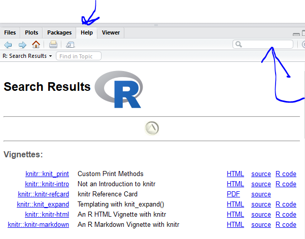
The help() function and ? help operator in R provide access to the documentation pages for R functions, data sets, and other objects, both for packages in the standard R distribution and for contributed packages. To do so type as follows

help({function})
help(package = {package name})

?{function}
?"{package name}"

Exercise

Look at the documentation for the seq function. What does seq do? Give an example of using seq with either the by or length.out argument.

Packages

While you can write your own functions, most functions you use will be part of a package. In R, the fundamental unit of shareable code is the package. A package bundles together code, data, documentation, and tests, and is easy to share with others. As of July 2018, there were over 14,000 packages available on the Comprehensive R Archive Network, or CRAN, the public clearing house for R packages. This huge variety of packages is one of the reasons that R is so successful.

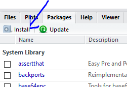
Installing a package using RStudio requires selecting the Install Packages Button in the Files, Plots, Packages Pane

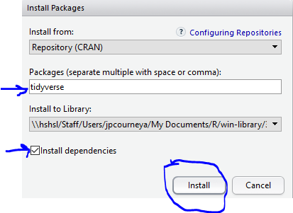
In the pop up box that results simply type the name of the package and check “install dependencies” and click Install

Its also possible for you to install and load packages from the console. Always make sure to put the package name in quotes when installing and setting dependencies = True

install.packages("tidyverse", dependencies = TRUE)    
library(tidyverse)

You only need to install a package once, but you need to reload it every time you start a new session.

Vectors

Vectors are probably the most used commonly used object type in R. “Vector” means different things in different fields (mathematics, geometry, biology), but in R a vector is a collection of values that are all of the same type (numbers, characters, etc.).

Data Types

There are numerous data types. Some of the other most common data types you will encounter are numeric data, character data and logical data. Vectors of one data type only are called atomic vectors. Read more about vectors and data types in the book R for Data Science

One of the most common ways to create a vector is to use the c() function - the “concatenate” or “combine” function. Inside the function you may enter one or more values; for multiple values, separate each value with a comma:

# Create the SNP gene name vector

snp_genes <- c("OXTR", "ACTN3", "AR", "OPRM1")

Vectors always have a mode and a length. You can check these with the mode() and length() functions respectively. Another useful function that gives both of these pieces of information is the str() (structure) function.

# Check the mode, length, and structure of 'snp_genes'
mode(snp_genes)

[1] "character"

length(snp_genes)

[1] 4

str(snp_genes)

 chr [1:4] "OXTR" "ACTN3" "AR" "OPRM1"

Vectors are quite important in R. Another data type that we will work with later in this lesson, data frames, are collections of vectors. What we learn here about vectors will pay off even more when we start working with data frames.

Creating and subsetting vectors

Let’s create a few more vectors to play around with:

# Some interesting human SNPs
# while accuracy is important, typos in the data won't hurt you here

snps <- c("rs53576", "rs1815739", "rs6152", "rs1799971")
snp_chromosomes <- c("3", "11", "X", "6")
snp_positions <- c(8762685, 66560624, 67545785, 154039662)

Once we have vectors, one thing we may want to do is specifically retrieve one or more values from our vector. To do so, we use bracket notation. We type the name of the vector followed by square brackets. In those square brackets we place the index (e.g. a number) in that bracket as follows:

# get the 3rd value in the snp vector
snps[3]

[1] "rs6152"

In R, every item your vector is indexed, starting from the first item (1) through to the final number of items in your vector. You can also retrieve a range of numbers:

# get the 1st through 3rd value in the snp vector

snps[1:3]

[1] "rs53576"   "rs1815739" "rs6152"

If you want to retrieve several (but not necessarily sequential) items from a vector, you pass a vector of indices; a vector that has the numbered positions you wish to retrieve.

# get the 1st, 3rd, and 4th value in the snp vector

snps[c(1, 3, 4)]

[1] "rs53576"   "rs6152"    "rs1799971"

There are additional (and perhaps less commonly used) ways of subsetting a vector (see these examples.

Also, several of these subsetting expressions can be combined:

# get the 1st through the 3rd value, and 4th value in the snp vector
# yes, this is a little silly in a vector of only 4 values.
snps[c(1:3,4)]

[1] "rs53576"   "rs1815739" "rs6152"    "rs1799971"

Adding to, removing, or replacing values in existing vectors

Once you have an existing vector, you may want to add a new item to it. To do so, you can use the c() function again to add your new value:

# add the gene "CYP1A1" and "APOA5" to our list of snp genes
# this overwrites our existing vector
snp_genes <- c(snp_genes, "CYP1A1", "APOA5")

We can verify that “snp_genes” contains the new gene entry

snp_genes

[1] "OXTR"   "ACTN3"  "AR"     "OPRM1"  "CYP1A1" "APOA5"

Using a negative index will return a version of a vector with that index’s value removed:

snp_genes[-6]

[1] "OXTR"   "ACTN3"  "AR"     "OPRM1"  "CYP1A1"

We can remove that value from our vector by overwriting it with this expression:

snp_genes <- snp_genes[-6]
snp_genes

[1] "OXTR"   "ACTN3"  "AR"     "OPRM1"  "CYP1A1"

We can also explicitly rename or add a value to our index using double bracket notation:

snp_genes[6]<- "APOA5"
snp_genes

[1] "OXTR"   "ACTN3"  "AR"     "OPRM1"  "CYP1A1" "APOA5"

Exercise: Examining and subsetting vectors

Answer the following questions to test your knowledge of vectors

Which of the following are true of vectors in R? A) All vectors have a mode or a length
B) All vectors have a mode and a length
C) Vectors may have different lengths
D) Items within a vector may be of different modes
E) You can use the c() to add one or more items to an existing vector
F) You can use the c() to add a vector to an existing vector

Solution

False - Vectors have both of these properties
True
True
False - Vectors have only one mode (e.g. numeric, character); all items in
a vector must be of this mode.
True
True

Logical Subsetting

There is one last set of cool subsetting capabilities we want to introduce. It is possible within R to retrieve items in a vector based on a logical evaluation or numerical comparison. For example, let’s say we wanted get all of the SNPs in our vector of SNP positions that were greater than 100,000,000. We could index using the ‘>’ (greater than) logical operator:

snp_positions[snp_positions > 100000000]

[1] 154039662

In the square brackets you place the name of the vector followed by the comparison operator and (in this case) a numeric value. Some of the most common logical operators you will use in R are:

Operator	Description
<	less than
<=	less than or equal to
>	greater than
>=	greater than or equal to
==	exactly equal to
!=	not equal to
!x	not x
a	b
a & b	a and b

The magic of programming

The reason why the expression snp_positions[snp_positions > 100000000] works can be better understood if you examine what the expression “snp_positions > 100000000” evaluates to:

snp_positions > 100000000

[1] FALSE FALSE FALSE  TRUE

The output above is a logical vector, the 4th element of which is TRUE. When you pass a logical vector as an index, R will return the true values:

snp_positions[c(FALSE, FALSE, FALSE, TRUE)]

[1] 154039662

If you have never coded before, this type of situation starts to expose the “magic” of programming. We mentioned before that in the bracket notation you take your named vector followed by brackets which contain an index: named_vector[index]. The “magic” is that the index needs to evaluate to a number. So, even if it does not appear to be an integer (e.g. 1, 2, 3), as long as R can evaluate it, we will get a result. That our expression snp_positions[snp_positions > 100000000] evaluates to a number can be seen in the following situation. If you wanted to know which index (1, 2, 3, or 4) in our vector of SNP positions was the one that was greater than 100,000,000?

We can use the which() function to return the indices of any item that evaluates as TRUE in our comparison:

which(snp_positions > 100000000)

[1] 4

Why this is important

Often in programming we will not know what inputs and values will be used when our code is executed. Rather than put in a pre-determined value (e.g 100000000) we can use an object that can take on whatever value we need. So for example:

snp_marker_cutoff <- 100000000
snp_positions[snp_positions > snp_marker_cutoff]

[1] 154039662

Ultimately, it’s putting together flexible, reusable code like this that gets at the “magic” of programming!

A few final vector tricks

Finally, there are a few other common retrieve or replace operations you may want to know about. First, you can check to see if any of the values of your vector are missing (i.e. are NA, that stands for not avaliable). Missing data will get a more detailed treatment later, but the is.NA() function will return a logical vector, with TRUE for any NA value:

snp_genes <- c("OXTR", "ACTN3", "AR", "OPRM1", "CYP1A1", NA, "APOA5")

is.na(snp_genes)

[1] FALSE FALSE FALSE FALSE FALSE  TRUE FALSE

sum(is.na(snp_genes))

[1] 1

Sometimes, you may wish to find out if a specific value (or several values) is present a vector. You can do this using the comparison operator %in%, which will return TRUE for any value in your collection that is in the vector you are searching:

# current value of 'snp_genes':
# chr [1:7] "OXTR" "ACTN3" "AR" "OPRM1" "CYP1A1" NA "APOA5"

# test to see if "ACTN3" or "APO5A" is in the snp_genes vector
# if you are looking for more than one value, you must pass this as a vector

snp_genes %in% c("ACTN3","APOA5")

[1] FALSE  TRUE FALSE FALSE FALSE FALSE  TRUE

Exercise 1

What data modes are the following vectors? a. snps
b. snp_chromosomes
c. snp_positions

Solution

mode(snps)

[1] "character"

mode(snp_chromosomes)

[1] "character"

mode(snp_positions)

[1] "numeric"

Exercise 2

Add the following values to the specified vectors: a. To the snps vector add: “rs662799”
b. To the snp_chromosomes vector add: 11
c. To the snp_positions vector add: 116792991

Solution

snps <- c(snps, "rs662799")
snps

[1] "rs53576"   "rs1815739" "rs6152"    "rs1799971" "rs662799"

snp_chromosomes <- c(snp_chromosomes, "11") # did you use quotes?
snp_chromosomes

[1] "3"  "11" "X"  "6"  "11"

snp_positions <- c(snp_positions, 116792991)
snp_positions

[1]   8762685  66560624  67545785 154039662 116792991

Exercise 3

Make the following change to the snp_genes vector:

Hint: Your vector should look like this in ‘Environment’: chr [1:7] "OXTR" "ACTN3" "AR" "OPRM1" "CYP1A1" NA "APOA5". If not recreate the vector by running this expression: snp_genes <- c("OXTR", "ACTN3", "AR", "OPRM1", "CYP1A1", NA, "APOA5")

Create a new version of snp_genes that does not contain CYP1A1 and then
Add 2 NA values to the end of snp_genes

Solution

snp_genes <- snp_genes[-5]
snp_genes <- c(snp_genes, NA, NA)
snp_genes

[1] "OXTR"  "ACTN3" "AR"    "OPRM1" NA      "APOA5" NA      NA

Exercise 4

Using indexing, create a new vector named combined that contains:

The the 1st value in snp_genes
The 1st value in snps
The 1st value in snp_chromosomes
The 1st value in snp_positions

Solution

combined <- c(snp_genes[1], snps[1], snp_chromosomes[1], snp_positions[1])
combined

[1] "OXTR"    "rs53576" "3"       "8762685"

Exercise 5

What type of data is combined?

Solution

typeof(combined)

[1] "character"

Key points

Effectively using R is a journey of months or years. Still you don’t have to be an expert to use R and you can start using and analyzing your data with with about a day’s worth of training
It is important to understand how data are organized by R in a given object type and how the mode of that type (e.g. numeric, character, logical, etc.) will determine how R will operate on that data.
Working with vectors effectively prepares you for understanding how data are organized in R.