Data Wrangling with R

An Introduction to the Tidyverse

Learning Objectives

By the end of this session, students will be able to:

Explain some benefits of learning R
Understand the difference between R and RStudio
Navigate RStudio
Define key R concepts and terminology.
Identify sources of documentation about R packages and functions
Apply commonly used tidyverse functions to a real data set
Becoming familiar with a typical workflow for exploring and wrangling data.

Why learn R?

R is free, open-source, and cross-platform. Anyone can inspect the source code to see how R works. Because of this transparency, there is less chance for mistakes, and if you (or someone else) find some, you can report and fix bugs. Because R is open source and is supported by a large community of developers and users, there is a very large selection of third-party add-on packages which are freely available to extend R’s native capabilities.
R code is great for reproducibility. Reproducibility is when someone else (including your future self) can obtain the same results from the same dataset when using the same analysis. R integrates with other tools to generate manuscripts from your code. If you collect more data, or fix a mistake in your dataset, the figures and the statistical tests in your manuscript are updated automatically.
R relies on a series of written commands, not on remembering a succession of pointing and clicking. If you want to redo your analysis because you collected more data, you don’t have to remember which button you clicked in which order to obtain your results; you just have to run your script again.
R is interdisciplinary and extensible With 10,000+ packages that can be installed to extend its capabilities, R provides a framework that allows you to combine statistical approaches from many scientific disciplines to best suit the analytical framework you need to analyze your data. For instance, R has packages for image analysis, GIS, time series, population genetics, and a lot more.
R works on data of all shapes and sizes. The skills you learn with R scale easily with the size of your dataset. Whether your dataset has hundreds or millions of lines, it won’t make much difference to you. R is designed for data analysis. It comes with special data structures and data types that make handling of missing data and statistical factors convenient. R can connect to spreadsheets, databases, and many other data formats, on your computer or on the web.
R produces high-quality graphics. The plotting functionalities in R are endless, and allow you to adjust any aspect of your graph to convey most effectively the message from your data.
R has a large and welcoming community. Thousands of people use R daily. Many of them are willing to help you through mailing lists and websites such as Stack Overflow, or on the RStudio community. Questions which are backed up with short, reproducible code snippets are more likely to attract knowledgeable responses.

Starting out in R

R is both a programming language and an interactive environment for data exploration and statistics.

Working with R is primarily text-based. The basic mode of use for R is that the user provides commands in the R language and then R computes and displays the result.

Downloading, Installing and Running R

Download
R can be downloaded from CRAN (The Comprehensive R Archive Network) for Windows, Linux, or Mac.

Install
Installation of R is like most software packages and you will be guided. Should you have any issues or need help you can refer to R Installation and Administration

Running
R can be launched from your software or applications launcher or When working at a command line on UNIX or Windows, the command R can be used for starting the main R program in the form R

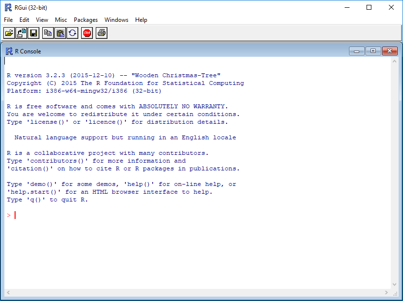
You will see a console similar to this appear:

While it is possible to work solely through the console or using a command line interface, the ideal environment to work in R is RStudio.

RStudio

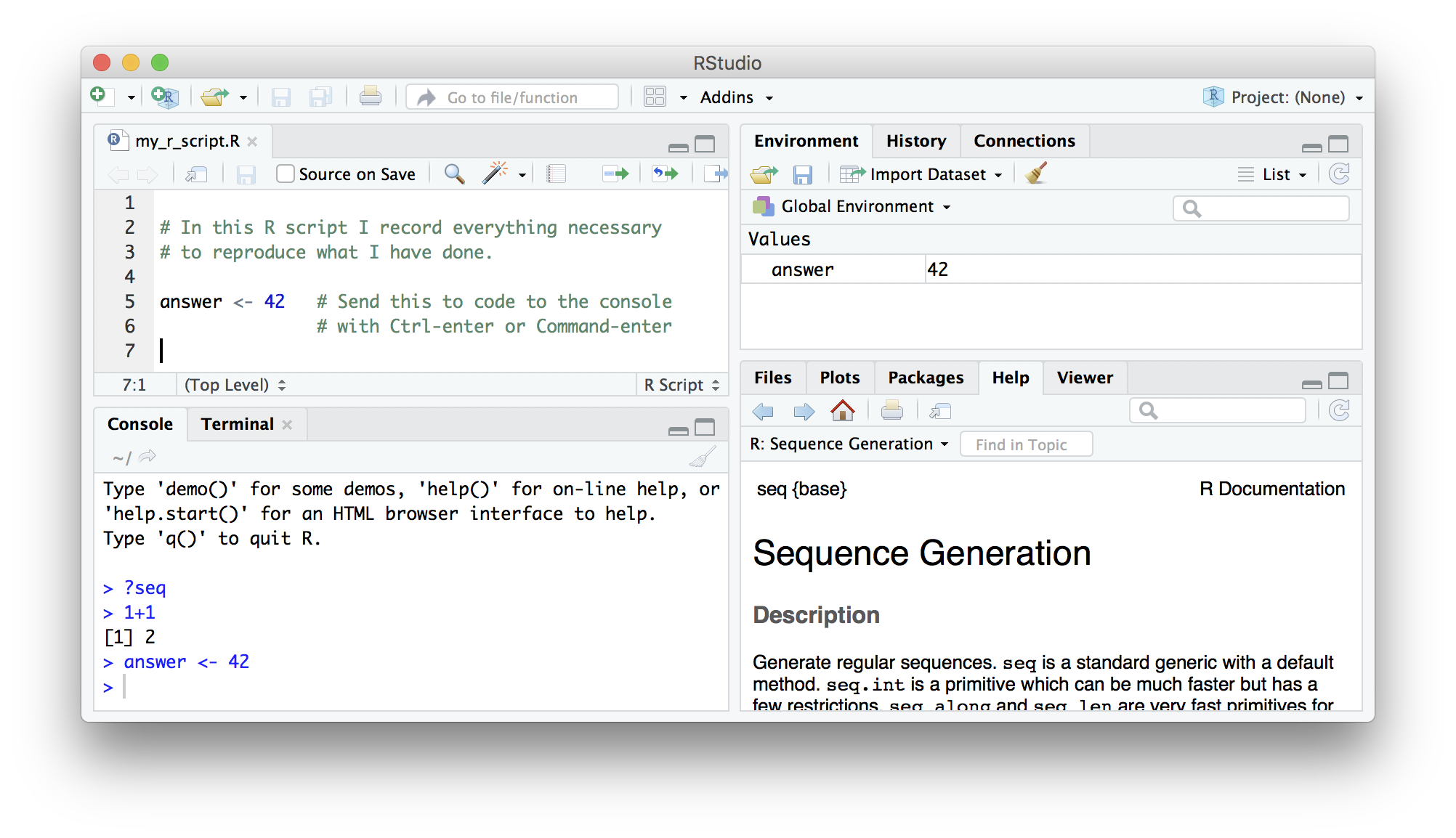
RStudio is a user interface for working with R. It is called an Integrated Development Environment (IDE): a piece of software that provides tools to make programming easier. RStudio acts as a sort of wrapper around the R language. You can use R without RStudio, but it<80><99>s much more limiting. RStudio makes it easier to import datasets, create and write scripts, and makes using R much more effective. RStudio is also free and open source. To function correctly, RStudio needs R and therefore both need to be installed on your computer.

RStudio is divided into four “panes”. The placement of these panes and their content can be customized (see menu, Tools -> Global Options -> Pane Layout).

The Default Layout is:

Top Left - Source: your scripts and documents
Bottom Left - Console: what R would look and be like without RStudio
Top Right - Environment/History: look here to see what you have done
Bottom Right - Files and more: see the contents of the project/working directory here, like your Script.R file

RStudio Projects

RStudio provides a useful feature called Projects which act like a container for your work. As you use R more, you will find it useful to make sure your files and environment for one real-world project are kept together and separate from other projects.

Let’s create a new project now.

Go to File > New Project
In Create project from menu choose Existing Directory
Browse to Desktop > Session01_DataWrangling
Select the check box that says Open in New Session

Follow Along at Home

Posit (RStudio) Cloud is a browser-based version of RStudio. It will allow you to use RStudio without needing to download anything to your computer. Posit Cloud automatically organizes things into Projects. You can also easily share your R projects with others.

Get Started:

Create your free RStudio Cloud account at https://posit.cloud/plans/free.
Go to the class project https://posit.cloud/content/8458222
Note the text that marks this as a Temporary Copy. Select the Save a Permanent Copy button to begin working!

R Scripts

A script is a text file in which you write your code. R scripts are generally recognized by the .R file extension. Scripts make it easy to re-run that code when you need to. In addition to code, your script can also have comments, which start with a # symbol. These comments make your script more human readable, but are ignored by the computer.

To get started in this lesson - open up the script in your RStudio Project called 01_DataWrangling.R

Welcome to the Tidyverse

In this lesson, we will be using a group of packages which are part of what is known as the tidyverse - “an opinionated collection of R packages designed for data science. All packages share an underlying design philosophy, grammar, and data structures.”¹, developed by Hadley Wickham.

What is a package?

As mentioned above, R is extensible and packages are the way to extend the base functionality of R. Each package is a collection of functions, code, data, and documentation. Packages are specialized to accomplish a particular set of tasks. Users can easily install packages from package repositories, such as the central repository CRAN (Comprehensive R Archive Network) and Bioconductor, an important source of bioinformatics packages.

The sheer number of R packages can seem overwhelming to a beginner and a common question we hear is, “But how do I know what package to use?”. One place is to start is to take a look at CRAN Task Views, which organizes packages by topic. You can also try an internet search like “How do I do X in R” and this will typically lead you to solutions that mention packages you need to accomplish the task.

One reason we are focusing on the tidyverse packages in this class is because they are so versatile and might be the only packages you need for much of what you want to do in R.

The tidyverse packages we will be using include:

readr for importing data into R
dplyr for handling common data wrangling tasks for tabular data
tidyr which enables you to swiftly convert between different data formats (long vs. wide) for plotting and analysis
lubridate for working with dates
ggplot2 for visualizing data (we’ll explore this package in the next session).

For the full list of tidyverse packages and documentation visit tidyverse.org You can install these packages individually, or you can install the entire tidyverse in one go.

Installing and loading packages

When you first install R on your computer, it comes with a set of built-in packages and functions collectively referred to as Base R. To add additional packages, you must first install that package, and then load it into your current session. If you are taking this workshop in person at the library, or using the class Posit Cloud project, the tidyverse has already been installed, so we just need to load it. You only need to install a package once on a system, but you will load it each time you start a new r session. If the package had not already been installed, we would install with a function called install.packages().

#install tidyverse if you haven't yet
#install.packages("tidyverse")

#load tidyverse
library(tidyverse)

Functions

install.packages() and library() are two examples of functions. Functions are one of the most important components of R code. A function is like a canned script. It usually takes some inputs, called arguments inside the parentheses that follow the name of the function, performs one or more tasks, and often returns some kind of output. The library() function takes the name of the package to load as it’s argument.

How do you know what arguments a function takes? For that you need to turn to the documentation of a particular package, or from within RStudio you can look up a function with ?function-name. Let’s try it with the library() function.

?library

This opens the help pane in the lower right corner of RStudio. The documentation provides you with all the arguments and any default values, along with explanations of the arguments. Here we see that the the library function has the argument package with no defaults.

What is Tidy Data?

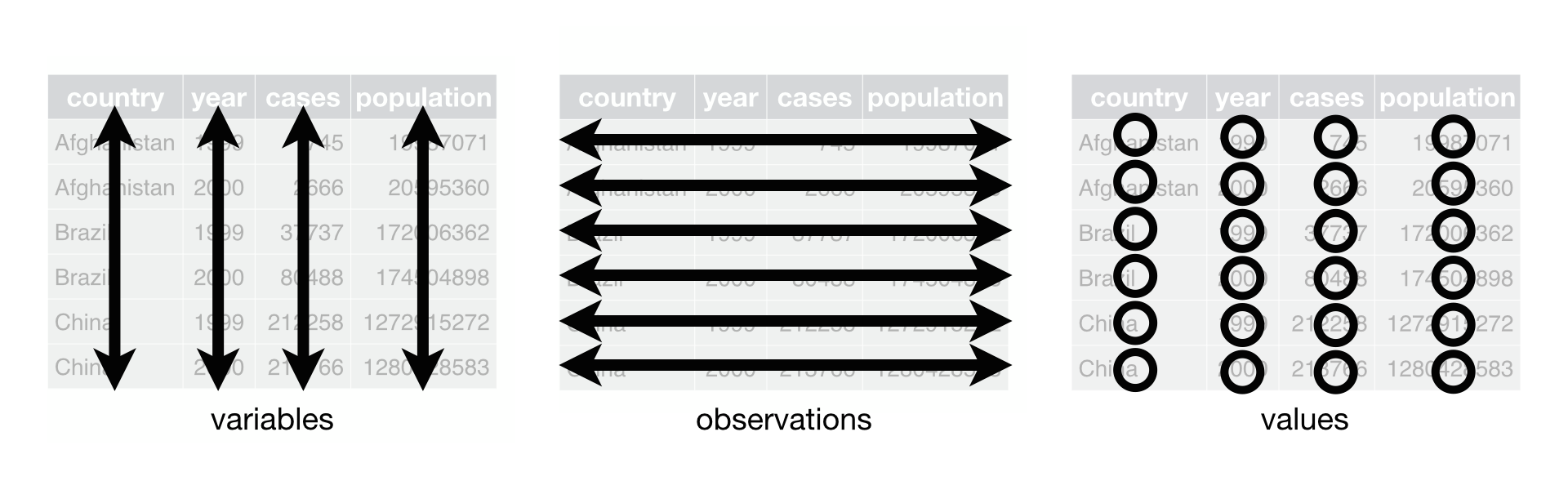
The tidyverse is so named from the concept of “tidy data”. Data is considered “tidy” if it follows three rules:

Each column is a variable
Each row is an observation
Each cell is a single value²

Data “in the wild” often isn’t tidy, but the tidyverse packages can help you create and analyze tidy datasets.

The Data for This Lesson

For this lesson we will be using data which comes from Project Tycho - an open data project from the University of Pittsburgh which provides standardized datasets on numerous diseases to aid global health research.

Throughout this lesson, we will be using a dataset from Project Tycho featuring historical counts of measles cases in the U.S.. We want to clean and present this data in a way that makes it easy to see how measles cases fluctuated over time.

A useful feature of Project Tycho data is their use of a common set of variables. Read more about their data format.

Importing data

Now,that the tidyverse is loaded, we can use it to import some data into our RStudio session. We are using a function from the readr package called read_csv(). This function takes as an argument the path to where the file is located. Let’s start by reading in measles_us file in the /data folder.

read_csv("data/measles_us.csv")

Rows: 422051 Columns: 15
-- Column specification --------------------------------------------------------
Delimiter: ","
chr (11): ConditionName, PathogenName, CountryName, CountryISO, Admin1Name, ...
dbl  (3): ConditionSNOMED, PartOfCumulativeCountSeries, CountValue
lgl  (1): DiagnosisCertainty

i Use `spec()` to retrieve the full column specification for this data.
i Specify the column types or set `show_col_types = FALSE` to quiet this message.

# A tibble: 422,051 x 15
   ConditionName ConditionSNOMED PathogenName  CountryName CountryISO Admin1Name
   <chr>                   <dbl> <chr>         <chr>       <chr>      <chr>     
 1 Measles              14189004 Measles virus UNITED STA~ US         WISCONSIN 
 2 Measles              14189004 Measles virus UNITED STA~ US         WISCONSIN 
 3 Measles              14189004 Measles virus UNITED STA~ US         WISCONSIN 
 4 Measles              14189004 Measles virus UNITED STA~ US         WISCONSIN 
 5 Measles              14189004 Measles virus UNITED STA~ US         WISCONSIN 
 6 Measles              14189004 Measles virus UNITED STA~ US         WISCONSIN 
 7 Measles              14189004 Measles virus UNITED STA~ US         WISCONSIN 
 8 Measles              14189004 Measles virus UNITED STA~ US         WISCONSIN 
 9 Measles              14189004 Measles virus UNITED STA~ US         WISCONSIN 
10 Measles              14189004 Measles virus UNITED STA~ US         WISCONSIN 
# i 422,041 more rows
# i 9 more variables: Admin1ISO <chr>, Admin2Name <chr>, CityName <chr>,
#   PeriodStartDate <chr>, PeriodEndDate <chr>,
#   PartOfCumulativeCountSeries <dbl>, DiagnosisCertainty <lgl>,
#   SourceName <chr>, CountValue <dbl>

But doing this just gives us a preview of the data in the console. To really use the data, we need to assign it to an object. An object is like a container for a numerical value, string, data set, image, and much more. Just about everything in R is an object. You might liken them to variables in other programming languages or in math. We create an object, by giving our data a name and use the assignment operator, which looks like an arrow <-. You can manually type in the lesser than sign < and hyphen -, or use the keyboard shortcut Alt + -.

Let’s call our new object measles_us. Object names should be short and easy to understand. They can’t have spaces, so you’ll want to separate multiple words with a underscore, or by using camel case. Object names also need to start with a letter not a number, and it’s best to avoid using names of common functions.

measles_us <- read_csv("data/measles_us.csv")

When you create an object, it shows up in your environment pane (the upper right panel). If we check our environment pane, we should now see an object called measles_us.

Let’s do the same for the states.csv file.

states <- read_csv(file = "data/states.csv")

Rows: 50 Columns: 3
-- Column specification --------------------------------------------------------
Delimiter: ","
chr (3): name, division, region

i Use `spec()` to retrieve the full column specification for this data.
i Specify the column types or set `show_col_types = FALSE` to quiet this message.

Exploring and Summarizing data

Data wrangling, also known as data cleaning or data munging, involves preparing raw data for analysis by transforming it into a more useful format. This process includes detecting and correcting errors, handling missing values, and reorganizing data for analysis. Using the tidyverse, we can streamline these tasks efficiently. After importing the data, you’ll typically start by exploring it, identifying patterns, and making necessary adjustments to prepare it for visualization and further analysis. This foundational step ensures that your data is accurate, consistent, and ready for insightful exploration.

Vectors and Data Frames and Tibbles oh my!

First, it’s important to understand the type of object we just created. In R, tabular data like you find in a spreadsheet is stored in a data frame, one of the fundamental data structures in R. A data frame is a rectangular, two-dimensional data structure. That is, it has both columns and rows. Data frames can store multiple data types, such as numeric, character, and logical data, also known as classes.

A tibble is a tidyverse version of the standard R data frame. For our purposes, the differences are minor enough that we can generally use the terms interchangeably, but to be precise, we will be working with tibbles in this lesson. All tibbles are data frames, but not all data frames are tibbles.

Another important R data structure is a vector. A vector is a one-dimensional data structure. That is, it is simply a sequence of elements. A vector can have only one data type. Data frames are created from multiple vectors, that is, each column in a data frame is a vector of the same length.

Base R functions for exploring data

View() opens the data as a file in your documents pane.This is a good way to see the data in a familiar spreadsheet-like format.

View(measles_us)

Use summary() to look at each column and find the data type and interquartile range for numeric data.

summary(measles_us)

Missing data

Sometimes we get data with a large number of missing values. It can be helpful to know where data is missing before attempting to do any further analysis. R uses NA to indicate missing values. We can use the function is.na() to test for the presence of NAs in our data.is.na() will return a vector of values TRUE or FALSE. TRUE if the value is NA, FALSE if it is not. When we examined our data with the View function, we might have noticed that the first several values in Admin2Name column are missing (NA). We might want to know how many missing values total are in that column.

is.na(measles_us$Admin2Name)

After running this code you should see TRUE printed out repeatedly in the console. R is running through that column and printing TRUE whenever it runs into a missing value. But this still does not help us get the total number of NAs. To do that we need to nest the above code in another function sum().

sum(is.na(measles_us$Admin2Name))

[1] 198104

sum() treats each each TRUE as a 1 and each FALSE as a 0. In that column there are 198104 out of 422051

But, if you have a lot of variables (columns), it would be a pain to do this for each one. So instead we can use a similar function colSums

colSums(is.na(measles_us))

              ConditionName             ConditionSNOMED 
                          0                           0 
               PathogenName                 CountryName 
                          0                           0 
                 CountryISO                  Admin1Name 
                          0                           0 
                  Admin1ISO                  Admin2Name 
                          0                      198104 
                   CityName             PeriodStartDate 
                     198104                           0 
              PeriodEndDate PartOfCumulativeCountSeries 
                          0                           0 
         DiagnosisCertainty                  SourceName 
                     422051                           0 
                 CountValue 
                          0

`tidyverse` functions for exploring data

The glimpse() function which is part of the tidyverse package tibble, lets you see the column names and data types clearly.

glimpse(measles_us)

distinct() returns the distinct rows in a tibble. It can be used on a column to return the distinct values in that column. The first argument you supply is the tibble object. Subsequent arguments include the variables you want to count.

distinct(measles_us, ConditionName)

# A tibble: 1 x 1
  ConditionName
  <chr>        
1 Measles

distinct(measles_us, Admin1Name)

# A tibble: 56 x 1
   Admin1Name
   <chr>     
 1 WISCONSIN 
 2 OHIO      
 3 MICHIGAN  
 4 NEVADA    
 5 NEW JERSEY
 6 WASHINGTON
 7 DELAWARE  
 8 KENTUCKY  
 9 WYOMING   
10 INDIANA   
# i 46 more rows

count() is similar to distinct() but also returns the number of observations (i.e. rows) for each of those distinct values. The first argument you supply is the tibble object. Subsequent arguments include the variables you want to count.

 count(measles_us, Admin1Name)

# A tibble: 56 x 2
   Admin1Name               n
   <chr>                <int>
 1 ALABAMA               7458
 2 ALASKA                1869
 3 AMERICAN SAMOA         118
 4 ARIZONA               4685
 5 ARKANSAS              5643
 6 CALIFORNIA           14354
 7 COLORADO              8042
 8 CONNECTICUT          10816
 9 DELAWARE              4507
10 DISTRICT OF COLUMBIA  5027
# i 46 more rows

Make code flow with the pipe %>%

Before we go any further - I want to introduce you to an important time-saving symbol in R called the pipe %>% (CTRL + SHIFT + M). The pipe allows you to take the output of the left-hand expression and make it the input of the right-hand expression. It allows you to chain together multiple functions and avoid nesting. With the pipe, we can rewrite the above code as follows:

measles_us %>% 
  count(Admin1Name)

# A tibble: 56 x 2
   Admin1Name               n
   <chr>                <int>
 1 ALABAMA               7458
 2 ALASKA                1869
 3 AMERICAN SAMOA         118
 4 ARIZONA               4685
 5 ARKANSAS              5643
 6 CALIFORNIA           14354
 7 COLORADO              8042
 8 CONNECTICUT          10816
 9 DELAWARE              4507
10 DISTRICT OF COLUMBIA  5027
# i 46 more rows

In many tidyverse functions, the first argument is the name of the data frame you’re applying the function to. So when you use the pipe, you’ll generally start a line of code with the name of a tibble. One benefit you might notice right away, is that when we use the pipe, RStudio will supply the column names which helps to reduce typing and typos.

Try it Yourself!

CHALLENGE

Now let’s try exploring the states tibble in our environment

Use glimpse() to inspect the columns and data types in the dataset.
Use distinct() to find out the distinct values in the region column.
Using count(), find out how many states are in each region.
Using count(), find out how many states are in each region AND division. HINT: You can add additional column names to distinct() and count() to look at combinations of columns.

Solution

glimpse(states)
states %>% distinct(region)
states %>% count(region)
states %>% count(region, division)

Subsetting data with `select()` and `filter()`

Real data sets can be quite large. So, once you’ve explored your data, you may want to start trimming it down to just the variables and conditions you’re interested in. In this section, we’ll look at two functions from the tidyverse package called dplyr: select() which lets you choose columns (variables) and filter() which lets you choose rows. (Note: dplyr is known for using easy to understand verbs for its function names.)

`select()`

select() lets you choose columns by name. The syntax of this function is similar to the the ones we’ve already learned count() and distinct(). We need to supply the function with the name of the tibble and the columns. This will create a new tibble with just those columns.

As with all tidyverse functions, we can use %>% to make this easier.

measles_us %>% 
select(Admin1Name, CountValue)

# A tibble: 422,051 x 2
   Admin1Name CountValue
   <chr>           <dbl>
 1 WISCONSIN          85
 2 WISCONSIN         120
 3 WISCONSIN          84
 4 WISCONSIN         106
 5 WISCONSIN          39
 6 WISCONSIN          45
 7 WISCONSIN          28
 8 WISCONSIN         140
 9 WISCONSIN          48
10 WISCONSIN          85
# i 422,041 more rows

If you want to select several columns that are next to each other, you can use : to specify a range, rather than writing each name out separately.

measles_us %>% 
select( ConditionName:Admin1ISO)

# A tibble: 422,051 x 7
   ConditionName ConditionSNOMED PathogenName  CountryName CountryISO Admin1Name
   <chr>                   <dbl> <chr>         <chr>       <chr>      <chr>     
 1 Measles              14189004 Measles virus UNITED STA~ US         WISCONSIN 
 2 Measles              14189004 Measles virus UNITED STA~ US         WISCONSIN 
 3 Measles              14189004 Measles virus UNITED STA~ US         WISCONSIN 
 4 Measles              14189004 Measles virus UNITED STA~ US         WISCONSIN 
 5 Measles              14189004 Measles virus UNITED STA~ US         WISCONSIN 
 6 Measles              14189004 Measles virus UNITED STA~ US         WISCONSIN 
 7 Measles              14189004 Measles virus UNITED STA~ US         WISCONSIN 
 8 Measles              14189004 Measles virus UNITED STA~ US         WISCONSIN 
 9 Measles              14189004 Measles virus UNITED STA~ US         WISCONSIN 
10 Measles              14189004 Measles virus UNITED STA~ US         WISCONSIN 
# i 422,041 more rows
# i 1 more variable: Admin1ISO <chr>

Now, let<80><99>s think through which columns we want for our analysis and save this to a new object called measles_select. It<80><99>s always a good idea to create new objects when you make major changes to your data.

For this exercise, we want to look at trends in number of measles cases over time. To do that, we<80><99>ll need to keep our CountValue variable, as and the date variables (PeriodStartDate and PeriodEndDate), as well as the PartOfCumulativeCountSeries variable, which will help us understand how to use the dates (more on this later). The first five columns each have only one value. So it might be redundant to keep those, although if we were combining them with other Project Tycho datasets they could be useful. It might be interesting to get a state-level view of the data, so let<80><99>s keep Admin1Name. But we saw that there are a number of missing values in our Admin2Name and CityName variables, so they might not be very useful for our analysis.

measles_select <-
  measles_us %>%
    select(
     Admin1Name,
     PeriodStartDate,
     PeriodEndDate,
     PartOfCumulativeCountSeries,
     CountValue
)

Sometimes when receive a data set or start working with data, you may find that the column names are overly long or not very descriptive or useful, and it may be necessary to rename them. For this, we can use the rename() function. Like naming objects, you should use a simple, descriptive, relatively short name without spaces for your column names. Let’s rename Admin1Name to State to make that more meaningful to us. rename() has the syntax rename(newColumnName = OldColumnName).

measles_select <-
  measles_select %>% 
    rename(state = Admin1Name)

Note that in this case, we are overwriting our original object with the new name instead of creating a new one!

`filter()`

While select() acts on columns, filter() acts on rows. filter() takes the name of the tibble and one or more logical conditions as arguments.

measles_md <- measles_select %>% 
  filter(state == "MARYLAND")

Here we are saying keep all the rows where the value in the state column is “MARYLAND”. Note the use of the double equals sign == versus the singular = sign. The double equal sign is a logical operator. The logical operators are:

operator	meaning
==	exactly equal
!=	not equal to
<	less than
<=	less than or equal to
>	greater than
>=	greater than or equal to
x\|y	x or y
x&y	x and y
!x	not x

Note that after running our code, our resulting tibble (our new object measles_md) has 7246 observations (rows) while our original tibble had 422051.

Warning

When matching strings you must be exact. R is case-sensitive. So state == "Maryland" or state == "maryland" would return 0 rows.

You can add additional conditions to filter by, separated other logical operators like &, >, and >.

Below we want just the rows for Maryland, and only include periods where the count was more than 500 reported cases. Note that while you need quotation marks around character data, you do not need them around numeric data.

measles_select %>%
  filter(state == "MARYLAND" & CountValue > 500)

# A tibble: 328 x 5
   state    PeriodStartDate PeriodEndDate PartOfCumulativeCountSeries CountValue
   <chr>    <chr>           <chr>                               <dbl>      <dbl>
 1 MARYLAND 1/29/1928       2/4/1928                                0        504
 2 MARYLAND 2/5/1928        2/11/1928                               0        563
 3 MARYLAND 2/12/1928       2/18/1928                               0        696
 4 MARYLAND 2/19/1928       2/25/1928                               0        750
 5 MARYLAND 2/26/1928       3/3/1928                                0       1012
 6 MARYLAND 3/4/1928        3/10/1928                               0        951
 7 MARYLAND 3/11/1928       3/17/1928                               0       1189
 8 MARYLAND 3/18/1928       3/24/1928                               0       1163
 9 MARYLAND 3/25/1928       3/31/1928                               0       1020
10 MARYLAND 4/1/1928        4/7/1928                                0        753
# i 318 more rows

Here, we joined together 2 conditions with the & logical operator. Then we piped that resulting tibble to count() which remember takes a tibble as its first argument.

What if we wanted to filter our tibble to include just the 50 states and no territories? We sure would not have to write out an expression for each state, or even all the territories.

# we can avoid verbose code like this with %in%

measles_select %>% 
filter(state == "MARYLAND" & state == "DELAWARE" & state == "Pennsylvania")

# A tibble: 0 x 5
# i 5 variables: state <chr>, PeriodStartDate <chr>, PeriodEndDate <chr>,
#   PartOfCumulativeCountSeries <dbl>, CountValue <dbl>

Luckily, We can filter based on a vector of values with the %in% operator (remember we can think of a vector as a column of data). So, we can write some code to filter our data based on list of state names in our states tibble.

measles_states_only <-
  measles_select %>% 
  filter(state %in% states$name)

Let’s save this output to a new object measles_states_only. Notice how we now have fewer rows than we had in our measles_select object.

We could alternatively have used negation with the names of the values we specifically wanted to exclude.

measles_states_only <- measles_select %>% 
  filter(!state %in% c("PUERTO RICO", "GUAM", "AMERICAN SAMOA", "NORTHERN MARIANA ISLANDS", "VIRGIN ISLANDS, U.S.", "DISTRICT OF COLUMBIA"))

Great! Our dataset is really shaping up. Let’s also take a closer look at our date columns. If you look at the first several rows, it looks like each row of our dataset represents about a discrete week of measles case counts. But (as you can read in the Tycho data documentation) there are actually two date series in this dataset - non-cumulative and cumulative. Which series a row belongs to is noted by the PartofCumulativeCountSeries, which as the value 0 if a row is non-cumulative, and 1 if the row is part of a cumulative count.

To keep things consistent. Let’s filter our tibble so we only have the non-overlapping discrete weeks.

measles_non_cumulative <- 
  measles_states_only %>% 
  filter(PartOfCumulativeCountSeries==0)

Once again, we have fewer rows than we started with.

Try it Yourself

CHALLENGE

Use select() to create a new tibble with just the name and division columns from the states tibble. Assign this to an object called us_divisions.
Use filter() to keep just the rows in the South Atlantic division of the us_divisions tibble. Assign this to an object called sa_division.
Use filter() to keep just the rows in the measles_non_cumulative tibble where the state matches one of the states in the name column of the sa_division tibble and where the CountValue is greater than 1000. Assign this to an object called measles_sa.

Solution

us_divisions <- states %>% select(name, division)
sa_division <- us_divisions %>% filter(division == "South Atlantic")
measles_sa <- measles_non_cumulative %>% filter(state %in% sa_division$name & CountValue > 1000)

Now let’s do some more with our date variables.

Changing and creating variables with `mutate()`

Let’s review the columns in our measles_states_only tibble

glimpse(measles_non_cumulative)

Rows: 332,138
Columns: 5
$ state                       <chr> "WISCONSIN", "WISCONSIN", "WISCONSIN", "WI~
$ PeriodStartDate             <chr> "11/20/1927", "11/27/1927", "12/4/1927", "~
$ PeriodEndDate               <chr> "11/26/1927", "12/3/1927", "12/10/1927", "~
$ PartOfCumulativeCountSeries <dbl> 0, 0, 0, 0, 0, 0, 0, 0, 0, 0, 0, 0, 0, 0, ~
$ CountValue                  <dbl> 85, 120, 84, 106, 39, 45, 28, 140, 48, 85,~

We can see from this that the dates are being interpreted as character data. We want R to recognize them as dates. We can create new variables and adjust existing variables with the mutate() function.

mutate() takes as an argument the name and definition of the new column you’re creating. Note that if you use the same variable name as an existing variable name it overwrites that column. Otherwise, it will add a column to your tibble.

To change the variable to a date - we are using a date parsing function from another package called lubridate. mdy() takes a character string or number in month-day-year format (as we have here) and returns a formal date object in YYYY-MM-DD format. There are similar functions if the input date is in year-month-day ydm() or day-month-year dmy()

measles_non_cumulative <- measles_non_cumulative %>% 
mutate(PeriodStartDate = mdy(PeriodStartDate),
       PeriodEndDate = mdy(PeriodEndDate))

Note that you can mutate multiple columns at a time, separating each new column definition with a comma.

Now that R recognizes the date columns as Dates, we can do things like extract parts of the date, such as the year. Let’s create a separate Year column. Later we’ll be able to group our tibble by year for analysis.

measles_year <- 
  measles_non_cumulative %>% 
  mutate(Year=year(PeriodStartDate))

Grouping and Summarizing

Many data analysis tasks can be approached using the split-apply-combine paradigm: split the data into groups, apply some analysis to each group, and then combine the results. dplyr makes this very easy through the use of the group_by() function.

group_by() is often used together with summarize(), which collapses each group into a single-row summary of that group. group_by() takes as arguments the column names that contain the categorical variables for which you want to calculate the summary statistics.

How can we calculate the total number of measles cases for each year?

First we need to group our data by year using our new Year column.

yearly_count <-
  measles_year %>%
  group_by(Year)

yearly_count

# A tibble: 332,138 x 6
# Groups:   Year [96]
   state   PeriodStartDate PeriodEndDate PartOfCumulativeCoun~1 CountValue  Year
   <chr>   <date>          <date>                         <dbl>      <dbl> <dbl>
 1 WISCON~ 1927-11-20      1927-11-26                         0         85  1927
 2 WISCON~ 1927-11-27      1927-12-03                         0        120  1927
 3 WISCON~ 1927-12-04      1927-12-10                         0         84  1927
 4 WISCON~ 1927-12-18      1927-12-24                         0        106  1927
 5 WISCON~ 1927-12-25      1927-12-31                         0         39  1927
 6 WISCON~ 1928-01-01      1928-01-07                         0         45  1928
 7 WISCON~ 1928-01-08      1928-01-14                         0         28  1928
 8 WISCON~ 1928-01-15      1928-01-21                         0        140  1928
 9 WISCON~ 1928-01-22      1928-01-28                         0         48  1928
10 WISCON~ 1928-01-29      1928-02-04                         0         85  1928
# i 332,128 more rows
# i abbreviated name: 1: PartOfCumulativeCountSeries

When you inspect your new tibble, everything should look the same. Grouping prepares your data for summarize, but it does not do anything visually to the data.

Now let’s trying summarizing that data. summarize() condenses the value of the group values to a single value per group. Like mutate(), we provide the function with the name of the new column that will hold the summary information. In this case, we will use the sum() function on the CountValue column and put this in a new column called TotalCount. Summarize will drop the columns that aren’t being used.

yearly_count <-
  measles_year %>%
  group_by(Year) %>%
  summarise(TotalCount = sum(CountValue))

yearly_count

# A tibble: 96 x 2
    Year TotalCount
   <dbl>      <dbl>
 1  1906       2345
 2  1907      40199
 3  1908      54471
 4  1909      49802
 5  1910      86984
 6  1911      59171
 7  1912      64773
 8  1913     111431
 9  1914      56440
10  1915      93579
# i 86 more rows

A more useful view might be to look for yearly totals of case counts by state. We can group by two variables, Year, and then State.

yearly_count_state <-
  measles_year %>%
  group_by(Year, state) %>%
  summarise(TotalCount = sum(CountValue))

`summarise()` has grouped output by 'Year'. You can override using the
`.groups` argument.

yearly_count_state

# A tibble: 4,055 x 3
# Groups:   Year [96]
    Year state         TotalCount
   <dbl> <chr>              <dbl>
 1  1906 CALIFORNIA           224
 2  1906 CONNECTICUT           23
 3  1906 FLORIDA                4
 4  1906 ILLINOIS             187
 5  1906 INDIANA               20
 6  1906 KENTUCKY               2
 7  1906 MAINE                 26
 8  1906 MASSACHUSETTS        282
 9  1906 MICHIGAN             320
10  1906 MISSOURI             274
# i 4,045 more rows

Notice how the use of pipes really comes in handy here. It saved us from having to create and keep track of a number of intermediate objects.

Sorting datasets with `arrange()`

Which state in which year had the highest case count? To easily find out, we can use the function arrange(). One of the arguments must be the column you want to sort on.

yearly_count_state %>% arrange(TotalCount)

# A tibble: 4,055 x 3
# Groups:   Year [96]
    Year state       TotalCount
   <dbl> <chr>            <dbl>
 1  1925 NEVADA               0
 2  1937 MISSISSIPPI          0
 3  1938 MISSISSIPPI          0
 4  1939 MISSISSIPPI          0
 5  1940 MISSISSIPPI          0
 6  1940 NEVADA               0
 7  1941 MISSISSIPPI          0
 8  1944 MISSISSIPPI          0
 9  1945 MISSISSIPPI          0
10  1906 TEXAS                1
# i 4,045 more rows

By default, arrange sorts in ascending order. To sort by descending order we use together with the desc() function.

yearly_count_state %>% arrange(desc(TotalCount))

# A tibble: 4,055 x 3
# Groups:   Year [96]
    Year state        TotalCount
   <dbl> <chr>             <dbl>
 1  1938 PENNSYLVANIA     146467
 2  1941 PENNSYLVANIA     137180
 3  1938 ILLINOIS         127935
 4  1942 CALIFORNIA       116180
 5  1941 OHIO             114788
 6  1935 MICHIGAN         111413
 7  1941 NEW YORK         109663
 8  1938 MICHIGAN         109041
 9  1934 PENNSYLVANIA     107031
10  1938 WISCONSIN        104450
# i 4,045 more rows

Joining Datasets

Of course, looking at total counts in each state is not the most helpful metric without taking population into account. To rectify this, let’s try joining some historical population data with our measles data.

First we need to import the population data⁴.

hist_pop <-
  read_csv("data/Historical_Population_by_State.csv")

Rows: 107 Columns: 52
-- Column specification --------------------------------------------------------
Delimiter: ","
dbl (52): DATE, ALASKA, ALABAMA, ARKANSAS, ARIZONA, CALIFORNIA, COLORADO, CO...

i Use `spec()` to retrieve the full column specification for this data.
i Specify the column types or set `show_col_types = FALSE` to quiet this message.

Long vs Wide formats

Remember that for data to be considered “tidy”, it should be in what is called “long” format. Each column is a variable, each row is an observation, and each cell is a value. Our state population data is in “wide” format, because State Name is being treated as a variable, when it is really a value. Wide data is often preferable for human-readability, but is less ideal for machine-readability. To be able to join this data to our measles dataset, it needs to have 3 columns - Year, State Name, and Population.

We will use the package tidyr and the function pivot_longer to convert our population data to a long format, thus making it easier to join with our measles data.

Each column in our population dataset represents a state. To make it tidy we are going to reduce those to one column called State with the state names as the values of the column. We will then need to create a new column for population containing the current cell values. To remember that the population data is provided in 1000s of persons, we will call this new column pop1000.

pivot_longer() takes four principal arguments:

the data
cols are the names of the columns we use to fill the new values variable (or to drop).
the names_to column variable we wish to create from the cols provided.
the values_to column variable we wish to create and fill with values associated with the cols provided.

library(tidyr)
hist_pop_long <- hist_pop %>%
  pivot_longer(ALASKA:WYOMING,
               names_to = "state",
               values_to = "pop1000")

View(hist_pop_long)

Now our two datasets have similar structures, a column of state names, a column of years, and a column of values. Let’s join these two datasets by the state and year columns. Note that if both sets have the same column names, you do not need to specify anything in the by argument. We use a left join here which preserves all the rows in our measles dataset and adds the matching rows from the population dataset.

measles_joined<- yearly_count_state %>% 
  left_join(hist_pop_long, by=join_by(state, Year == DATE))

measles_joined

# A tibble: 4,055 x 4
# Groups:   Year [96]
    Year state         TotalCount pop1000
   <dbl> <chr>              <dbl>   <dbl>
 1  1906 CALIFORNIA           224    1976
 2  1906 CONNECTICUT           23    1033
 3  1906 FLORIDA                4     628
 4  1906 ILLINOIS             187    5309
 5  1906 INDIANA               20    2663
 6  1906 KENTUCKY               2    2234
 7  1906 MAINE                 26     729
 8  1906 MASSACHUSETTS        282    3107
 9  1906 MICHIGAN             320    2626
10  1906 MISSOURI             274    3223
# i 4,045 more rows

CHALLENGE

Use mutate() to calculate the rate of measles per 100,000 persons (remember population is given in 1000s).
Try joining measles_yearly_rates to states. What variable do you need to join by?

Solution

# 1. 
measles_yearly_rates <-
  measles_joined %>% 
  mutate(epi_rate = (TotalCount / pop1000)*100)

# 2. 
yearly_rates_joined <- measles_yearly_rates %>% 
  left_join(states, by = join_by(state == name))

Now our data is ready to be visualized!

Footnotes

https://www.tidyverse.org/↩︎
read more about tidy data https://cran.r-project.org/web/packages/tidyr/vignettes/tidy-data.html↩︎
image from R for Data Science https://r4ds.had.co.nz/tidy-data.html#fig:tidy-structure↩︎
population data retrieved from the FRED, the Federal Reserve Bank of St. Louis Economic Data, https://fred.stlouisfed.org/release/tables?rid=118&eid=259194↩︎

Learning Objectives

Why learn R?

Starting out in R

Downloading, Installing and Running R

RStudio

RStudio Projects

R Scripts

Welcome to the Tidyverse

Installing and loading packages

Functions

What is Tidy Data?

The Data for This Lesson

Importing data

Exploring and Summarizing data

Vectors and Data Frames and Tibbles oh my!

Base R functions for exploring data

tidyverse functions for exploring data

Try it Yourself!

Subsetting data with select() and filter()

select()

filter()

Try it Yourself

Changing and creating variables with mutate()

Grouping and Summarizing

Sorting datasets with arrange()

Joining Datasets

Long vs Wide formats

Footnotes

`tidyverse` functions for exploring data

Subsetting data with `select()` and `filter()`

`select()`

`filter()`

Changing and creating variables with `mutate()`

Sorting datasets with `arrange()`